Preprocessing
Objectives
- These slides are a three lecture series
- Part 1: Preprocessing related to all data types
- Part 2: Preprocessing specific to structural data
- Part 3: Preprocessing specific to functional data
Preprocessing
- General
- Structural
- Functional (fMRI)
- Task fMRI
- resting state fMRI
General
- Inhomogeneity correction
- Brain extraction
- Registration (also called [spatial] normalization)
- Spatial smoothing (applied downstream prior to analysis)
Structural
- Inhomogeneity correction
- Brain extraction
- Registration
- Tissue segmentation
- Volume estimation
- Surface reconstruction and cortical thickness estimation
- Spatial smoothing
Functional
- Inhomogeneity correction
- Brain extraction (via structural image)
- Registration
- Motion correction
- Slice timing correction
- Distortion correction (if field map available)
- Temporal filtering & confound regression
- Spatial smoothing
Inhomogeneity correction and brain extraction
- I won’t go into detail here, but know that these are preprocessing steps
- Inhomogeneity correction adjusts for systematic differences in the brightness of the image
- Brain extraction removes the skull, eyes, and surrounding tissue
Registration
Software listed are non-exhaustive.
Goal
- Brains are structurally very different
- Brains as functions/images can have different coordinate systems
- To compare features such as function or anatomy it helps if the coordinates are comparable
- Making coordinates comparable is the goal of registration
Terminology
- Input/moving image I(w), w \in \mathbb{R}^3
- Reference/target/template image R(v), v \in \mathbb{R}^3
- We want to find a transformation T such that
I(T(v)) \approx R(v)
General theory
- Estimation: minimizes cost (or maximizes similarity)
- Similarity metrics/cost functions
Least squares (images have the same scale) C\{ R(v), I(T(v))\} = \int_{v \subset \mathbb{R}^3} \{ I(T(v)) - R(v)\}^2 dv
Correlation (images on different scales)
Mutual information (images with different contrasts/distributions) \mathrm{MI}(R, I) = \sum_{r,i} \mathbb{P}_{RI}(r, i) \log \left( \frac{\mathbb{P}_{RI}(r, i)}{\mathbb{P}_R(r), \mathbb{P}_I(i)} \right)
where \mathbb{P}_{RI}(r, i): is the joint probability, and \mathbb{P}_R(r), \mathbb{P}_I(i) are the marginal probabilities
- Transformation computed to minimize \min_T C\{R(v), I(T(v))\}
- Some of these cost functions are convex given some assumptions on the images
- That would imply a global optimum, given some assumtions on I and R
- Those assumptions are not met, so many adhoc approaches are implemented1
- Penalty terms are often useful
- Registration is a challenging problem
Rigid-body
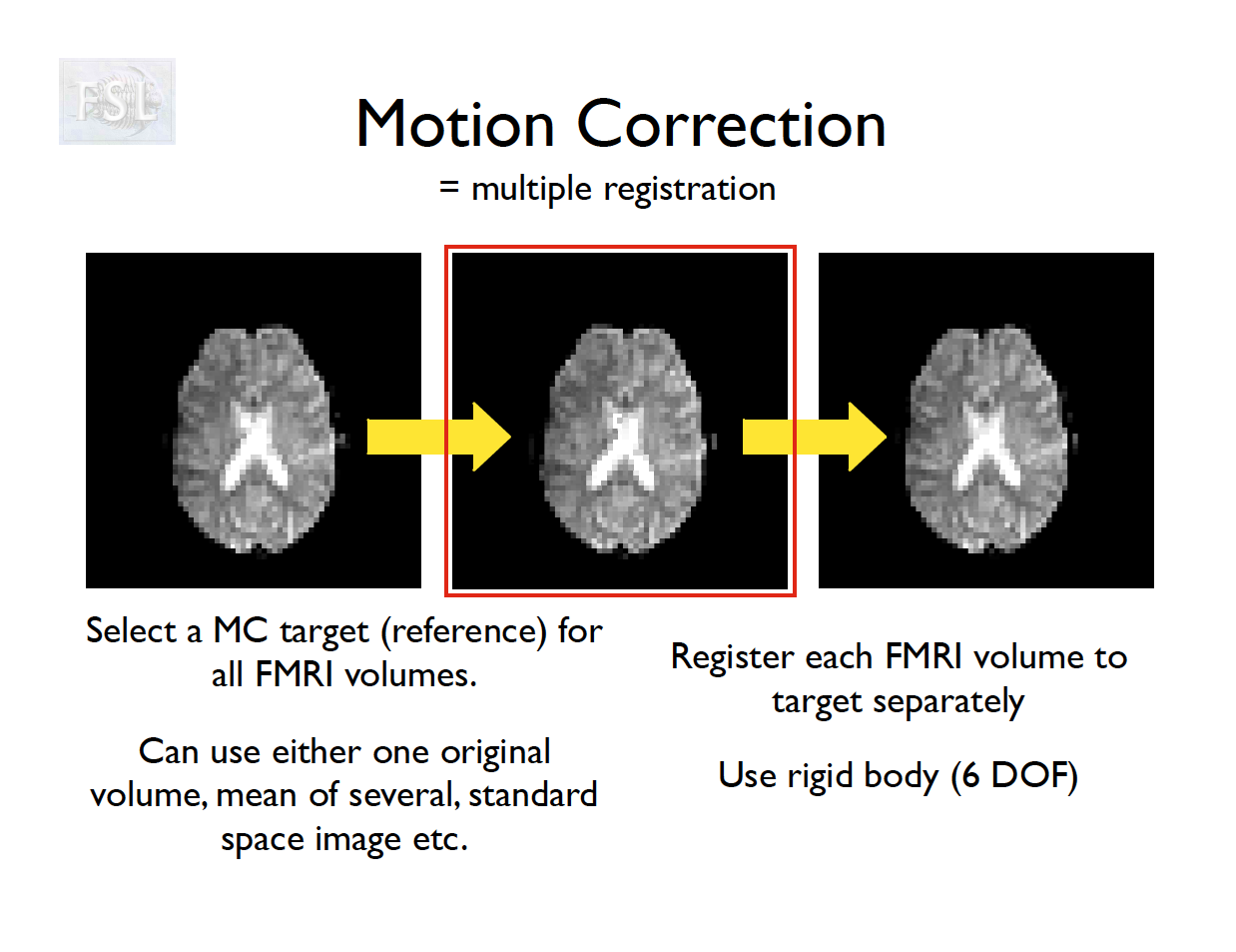
- Six parameter rigid registration
- Used to align functional images over time (motion correction)
- Also used to align images from the same participant collect in the same scan session.
- y = (y_1, y_2, y_3, 1) - template coordinates, x = (x_1, x_2, x_3, 1) input coordinates
- Appended with an intercept for transformation
- Can be described as the composition of four transformations
\begin{bmatrix} y_1 \\ y_2 \\ y_3\\ 1 \end{bmatrix} = T_4 T_3 T_2 T_1 \cdot \begin{bmatrix} x_1 \\ x_2 \\ x_3\\ 1 \end{bmatrix}
Translation of image T_4 = \begin{bmatrix} 1 & 0 & 0 & q_1 \\ 0 & 1 & 0 & q_2 \\ 0 & 0 & 1 & q_3\\ 0 & 0 & 0 & 1 \end{bmatrix}
Rotation around the x-axis:
T_1 = \begin{bmatrix} 1 & 0 & 0 & 0 \\ 0 & \cos(q_4) & \sin(q_4) & 0 \\ 0 & -\sin(q_4) & \cos(q_4) & 0\\ 0 & 0 & 0 & 1 \end{bmatrix}
Other rotations are defined similarly. See the reference above.
Affine (linear) registration
- Linear (Affine, actually) registration is 12 parameters
- The rigid body transformations are further augmented with “zoom” and “shear”
- All registrations should be invertible so that the reference can be moved to the space of the input
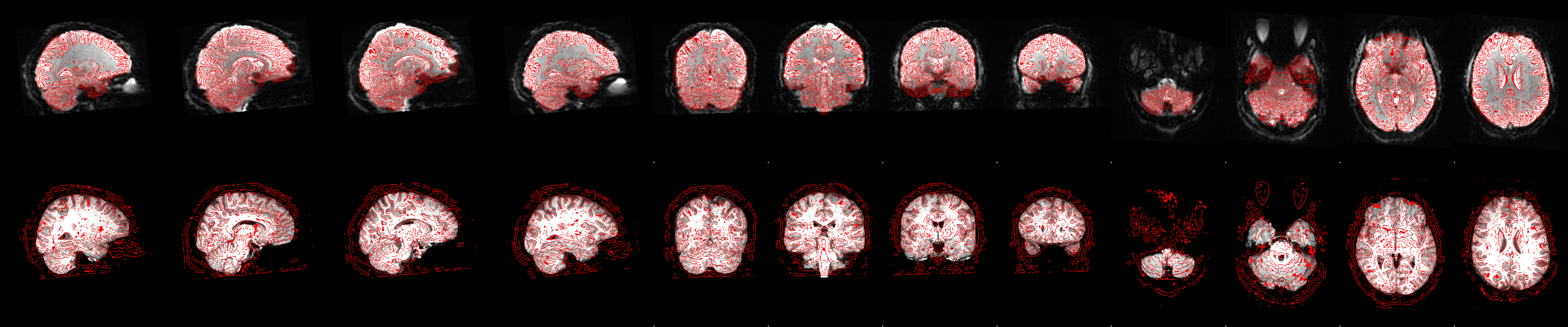
Example of registration results
Commands I ran:
fast -B images/simon_bc.nii.gz images/simon.nii.gz
bet images/simon_bc.nii.gz images/simonReg/simon_brain.nii.gz
# dof controls number of parameters 6 is rigid-body
flirt -in images/simonReg/simon_brain.nii.gz -ref images/MNI152_T1_1mm_brain.nii.gz -dof 6 -o images/simonReg/simon_brain_rigidReg.nii.gz -omat images/simonReg/rigidReg.txt
# defaults to 12 for affine transformation
flirt -in images/simonReg/simon_brain.nii.gz -ref images/MNI152_T1_1mm_brain.nii.gz -o images/simonReg/simon_brain_affineReg.nii.gz -omat images/simonReg/affineReg.txt
To view the results with the MNI template
To view transformation matrices
- Brain extraction
- Rigid-body
- Affine
Interpolation
- Images are measured on a grid, so applying the transformation T may require evaluation of the image, I, at locations not represented by a grid coordinate
- Interpolation computes I(T(v)) at non-grid locations
- Required for evaluating cost function and when applying the resulting transformation matrix.
- Interpolation methods
- Nearest neighbor interpolation is important when registering atlas images
- Atlas images are integer valued and nearest neighbor ensures output is integer valued
Nonlinear (deformable) registration
- Deformable registration allows different parts of the image to have a unique transformation matrix
- Called a deformation field \phi(x) such that y = \phi(x).
- Different approaches:
- B‑splines, diffeomorphisms (e.g., LDDMM, SyN), demons, finite-element
- Enforces smoothness, invertibility, and topology preservation via regularization.
- Typically linear transformation is estimated first, then function composition is used when estimating and evaluating the nonlinear transformation
- Composition avoids repeated interpolation of the image
- ANTs registration paper Avants et al (2009).
Visualize results
Registration to a template
- Common template images
- MNI template – MNI template is most common target for registration
- Study-specific template – in unique populations, often better to create a study-specific template
- e.g. Pediatric, aging, or patient populations
Registration output
HO_simon.nii.gz
MNI2simon.nii.gz
affineReg.txt
field.nii.gz
jacobian.nii.gz
rigidReg.txt
simon2MNI.nii.gz
simon_bet.nii.gz
simon_brain.nii.gz
simon_brain_affineReg.nii.gz
simon_brain_mixeltype.nii.gz
simon_brain_pve_0.nii.gz
simon_brain_pve_1.nii.gz
simon_brain_pve_2.nii.gz
simon_brain_pveseg.nii.gz
simon_brain_rigidReg.nii.gz
simon_brain_seg.nii.gz
simon_brain_to_MNI152_T1_1mm_brain.log
simon_brain_warpcoef.nii.gz
simon_nonlinearReg.nii.gz- Warp field – Tells the registration algorithm how much and what direction to move each voxel value
- Jacobian of the transformation – More accurately, the Jacobian determinant.
- The Jacobian is the (matrix valued) derivative of the warp field at each location. It describes how the voxel coordinates get moved at a given location
- The determinant of the transformation describes the amount the voxel has to move
Advanced registration topics
- Study specific templates
- Populations vary and a standard template might not be appropriate
- Examples: Kids or older adults
- Averages can be defined geometrically and modeled by covariates, which seems cool
References
- Human brain function online book (from the authors of SPM software
- Chapter 2 from HBF book
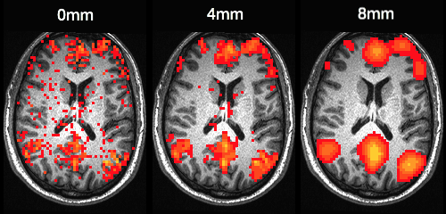
Spatial smoothing
A relatively simple processing step
Goal
- Registration is imperfect, applying spatial smoothing reduces between subject variability
- If there is voxel-level independent Gaussian noise, spatial smoothing will reduce the noise – math for this is relatively easy
- Smoothing is typically applied to images before statistical analysis
- Value at a smoothed voxel is a Gaussian weighted average of surrounding voxels in unsmoothed image
Terminology
- FWHM - full width at half maximum, typically in mm. Description of size of Gaussian kernel for smooth
- Sigma - \sigma = \frac{\mathrm{FWHM}}{2\sqrt{2\log(2)}}
Smoothing kernels CPAC pipeline
Structural preprocessing and output
C-PAC anatomical pipeline

Anatomical pipeline
Option/Alt + click to zoom in.
Segmentation
- Segmentation estimates gray/white matter, CSF/ventricles
- Variations on mixture models that incorporate priors and spatial dependence
# output from fsl_anat.
# Base image is the input data.
# Second image is the segmentation output
fsleyes data/RBC/HBN_BIDS/sub-NDARAA306NT2/ses-HBNsiteRU/anat/sub-NDARAA306NT2_ses-HBNsiteRU_acq-HCP_T1w.anat/T1.nii.gz data/RBC/HBN_BIDS/sub-NDARAA306NT2/ses-HBNsiteRU/anat/sub-NDARAA306NT2_ses-HBNsiteRU_acq-HCP_T1w.anat/T1_fast_pveseg.nii.gz
Volume estimation
Estimation of volumes of regions defined from an anatomical atlas.
Approaches:
- Registration - invert warp to map atlas to subject space
- Multi-atlas label fusion - Registration-based. Information from multiple manually labeled atlases can improve estimation
- Joint label fusion
- Probabilistic atlases/Bayesian models
- We can discuss these more as an advanced topic if there is interest
Volume estimation example
# invert the warp from subject space to template space
invwarp -w images/simonReg/simon2MNI.nii.gz -o images/simonReg/MNI2simon.nii.gz -r images/simonReg/simon_brain.nii.gz
# convert atlas to subject space. Use nearest neighbor interpolation
applywarp --i=/Users/vandeks/fsl/data/atlases/HarvardOxford/HarvardOxford-cort-maxprob-thr25-1mm.nii.gz --ref=images/simonReg/simon_brain.nii.gz --warp=images/simonReg/MNI2simon.nii.gz --out=images/simonReg/HO_simon.nii.gz --interp=nn
# visualize results on simon's brain
fsleyes images/simonReg/simon_brain.nii.gz images/simonReg/HO_simon.nii.gz
Code from ChatGPT to compute volumes.
# 2. Estimate voxel volume (assumes cubic mm)
voxel_volume=$(fslval ${ref_image} pixdim1)
voxel_volume=$(echo "${voxel_volume} * $(fslval ${ref_image} pixdim2) * $(fslval ${ref_image} pixdim3)" | bc -l)

# 3. Loop over atlas labels to count voxels and estimate volume
echo "Label,VoxelCount,Volume_mm3"
for label in {1..48}; do
  count=$(fslstats ${atlas_subj} -l $(($label - 1)) -u $label -V | awk '{print $1}')
  volume=$(echo "$count * $voxel_volume" | bc -l)
  echo "$label,$count,$volume"
done
Derivatives of the registration process
- Features of the registration process are informative of brain structure
- Probabilistic tissue segmentation: images can be analyzed across participants after registration to template space
- Determinant of the Jacobian: quantifies how much the image needed to be warped at that location to fit into the template space
- Voxel-based morphometry (VBM) combines Jacobian and tissue segmentation images to compare gray matter volume in template space
- Mechelli 2005 – Review of VBM
- Antonopoulos 2023 – Recent comparison of VBM methods
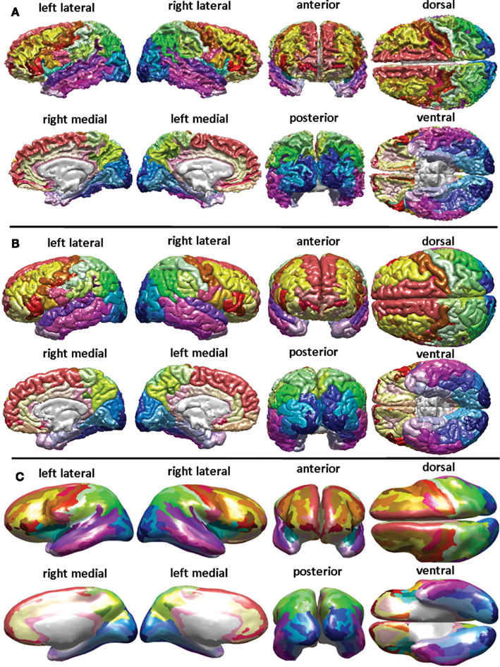
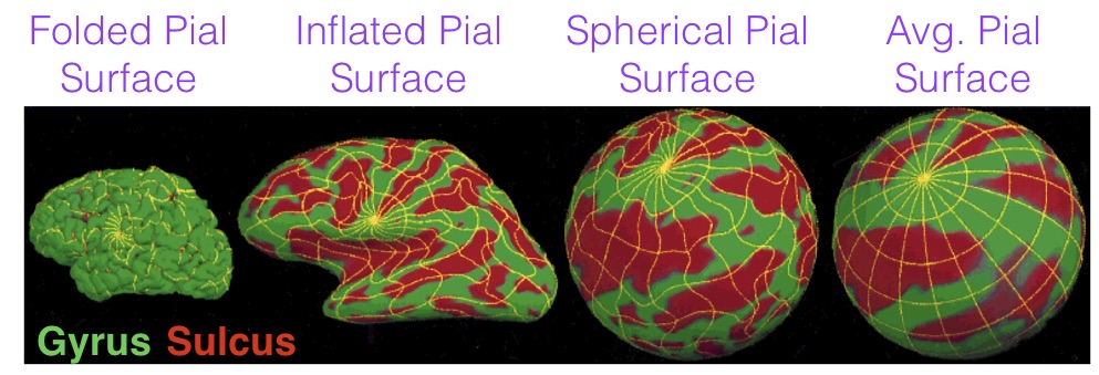
Cortical surface reconstruction
Freesurfer is among the most popular software for cortical surface reconstruction
- Allows projection of other data (e.g. fMRI) to the surface
- All analyses can be performed on the surface
- Registration in Freesurfer occurs on the surface manifold instead of in 3D
- Respects biology of the brain
- Smoothing is done on the surface – avoids smoothing over sulci
- Con: Does not include subcortex
Freesurfer software output
- Fully automated call, though it is not without errors/flaws
- A look at the Freesurfer output – maybe later
Functional preprocessing
- We will discuss common preprocessing steps and view some input/output in FSL
What are fMRI data?
- fMRI measures brain activity over time by detecting changes in blood oxygenation.
- fMRI data are a time series of 3D brain images, collected every 1–3 seconds (TR = repetition time).
- Each voxel (3D pixel) contains a time series reflecting fluctuations in signal intensity across the scan.
- The signal includes BOLD (Blood Oxygenation Level-Dependent) response
- Based on the fact that oxygenated and deoxygenated hemoglobin have different magnetic properties.
- Neural activity, increased blood flow, local increase in oxygenated blood, measurable signal change.
- Data are collected while participants
- Perform a task (task-based fMRI)
- Rest with eyes open/closed (resting-state fMRI)
- fMRI is indirect: it measures blood flow, not neural activity itself.
Functional preprocessing pipeline
- Scientists have developed many software tools for preprocessing
- The analysis pipeline is very sophisticated
- Teams have developed pipeline tools that make it easier to reproducibly preprocess the data
- Example CPAC functional pipeline

Functional pipeline
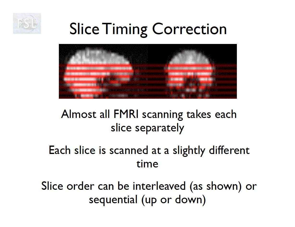
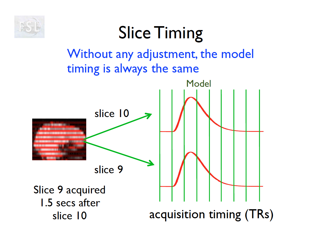
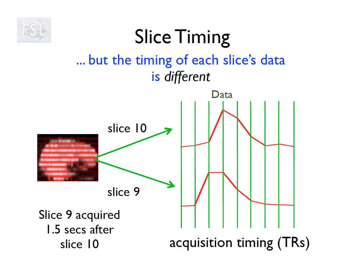
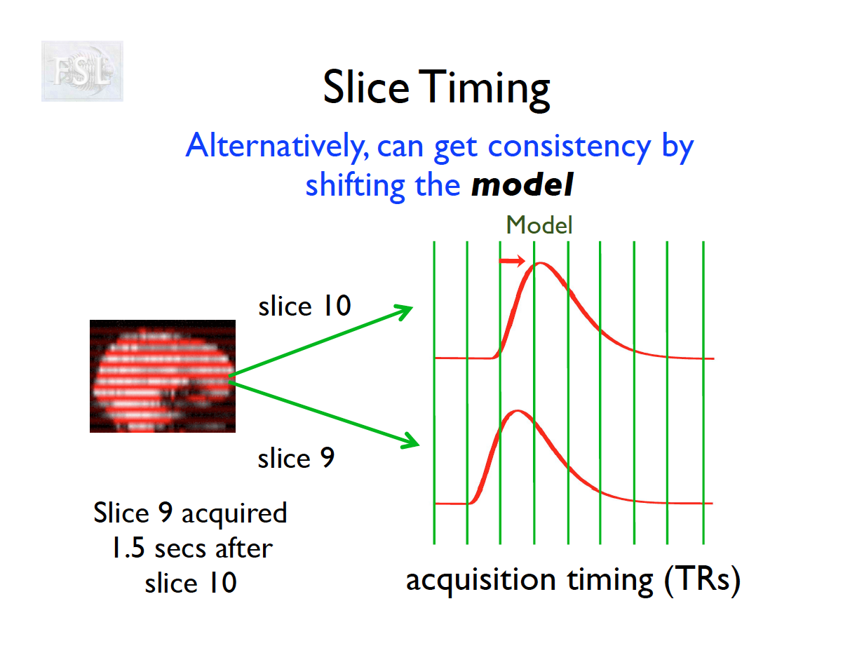
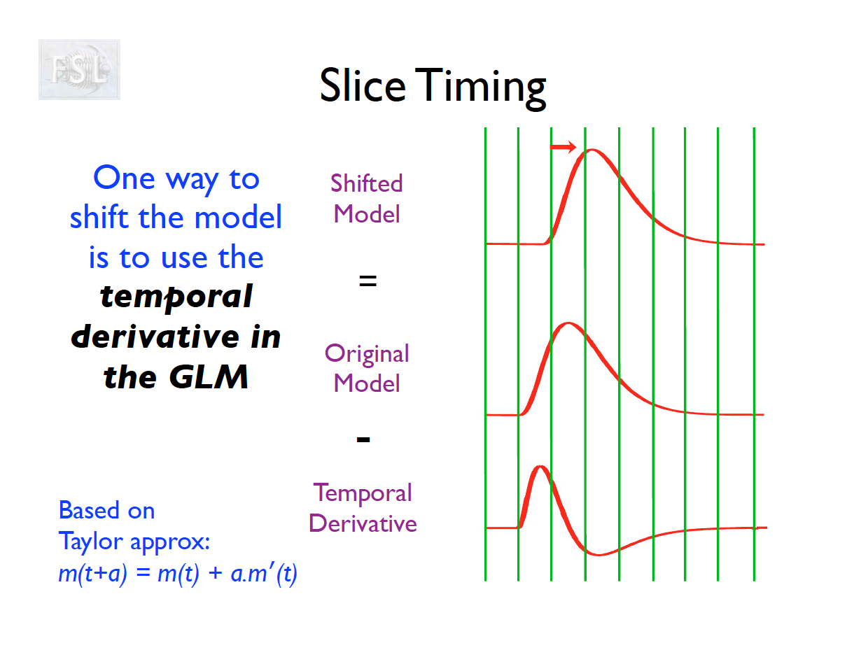
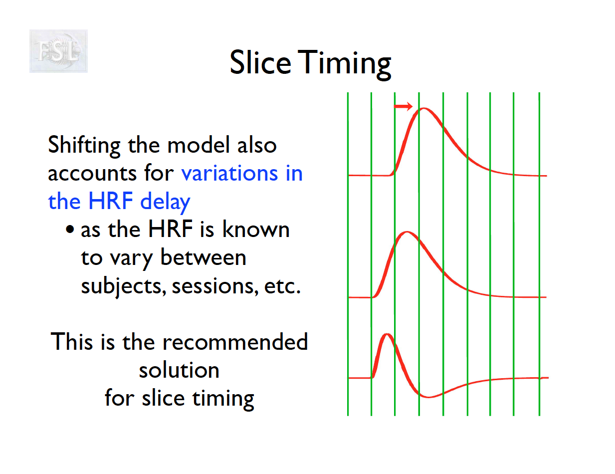
Slice Timing Correction
- fMRI data are collected sequentially in 2-d slices in the z-plane
- Over the course of one TR (repetition time; approximately 2 seconds [0.5-3 seconds] ), the time the first slice and the last slice are acquired is the TR length
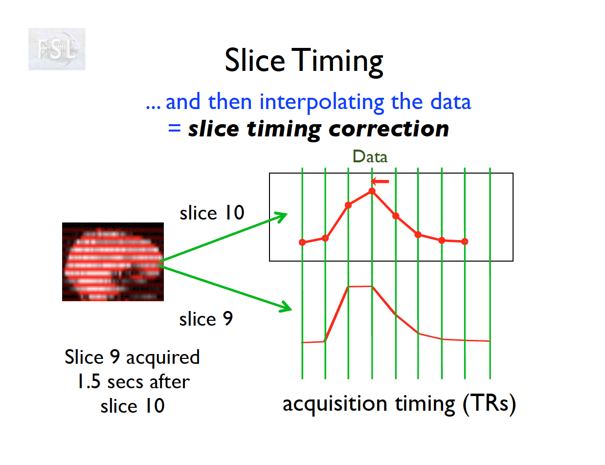
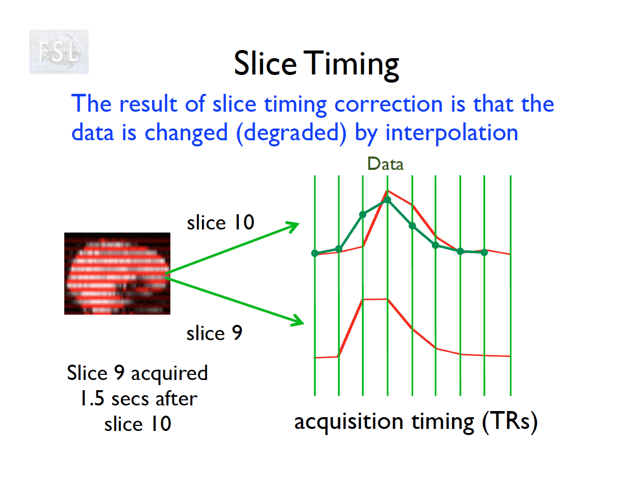
- Slice timing adjusts voxel intensities in each slice to a common acquisition reference (e.g., the first slice)
- Corrects timing offsets across the TR to align the hemodynamic response
- Uses interpolation (e.g., sinc, Fourier) based on slice order (alt‑z, seq, etc.)
- Multiband fMRI methods can acquire several slices simultaneously, reducing the TR.


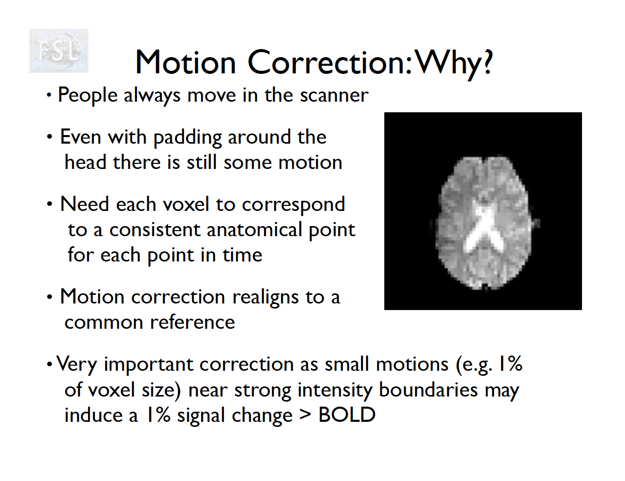
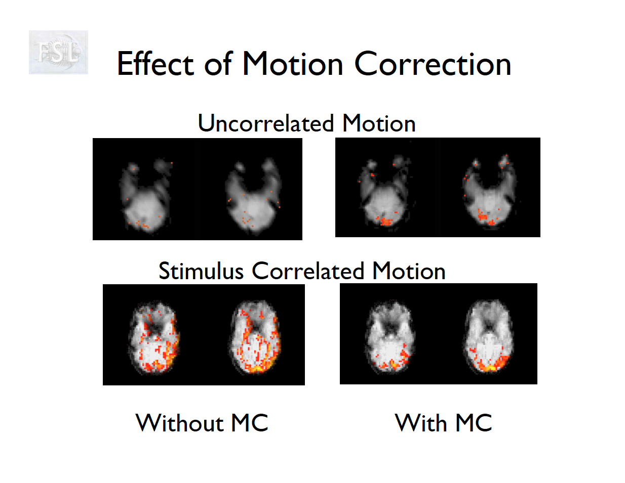
Motion correction
- The participant will move across the scan time
- Motion correction in FSL
- Align volumes to mean image
- Motion correction in AFNI (another software)
- Align volumes to mean image
- Realign again to newly computed mean for improved accuracy
Motion correction output
- Outputs:
- 6 motion parameters
- Mean framewise displacement (FD) and motion plots
- Motion parameter time series are used as covariates in first-level analysis
Motion parameters from Despicable Me

Temporal (high-pass) filtering
- Occurs as part of the first-level analysis to remove low-frequency drift
- Uses a discrete cosine transform on the time series and uses them as covariates in a regression (first-level analysis)
Implementation in FSL
- The cutoff in FSL’s high-pass filter (implemented via DCT regressors) is chosen based on the longest period of signal variation you want to keep relative to your task design.
How the DCT cutoff works
FEAT asks you for a high-pass filter cutoff (in seconds), e.g. 100s.
This is the minimum period length that will be modeled as noise.
All fluctuations slower than this period (i.e., longer trends) are captured by the DCT regressors and removed.
Faster fluctuations (shorter than this period) remain in the data/GLM.
Implementation: a set of cosine basis functions with periods ≥ cutoff are generated, spaced to cover the run length.
Rule of thumb in FSL: 2 × the longest inter-stimulus interval (ISI) / block length in your design.
Simon: Needs to be longer than the longest block length
Rationale: you want to preserve your task regressors of interest, but still remove very slow scanner drift.
Notes from ChatGPT about DCT-II used in FSL
FSL uses a Discrete Cosine Transform (DCT, Type II) basis set to model slow drifts.
If you have a run of length T seconds (N volumes × TR), then for each time point t = 0, 1, \dots, N-1:
X_{k}(t) \;=\; \cos\!\Bigg( \frac{\pi (t+0.5)k}{N} \Bigg), \quad k=0,1,\dots,N-1
This is the standard DCT-II form. Each k corresponds to a different frequency (periodicity).
Mapping cutoff to maximum period
The cutoff you choose in FEAT (e.g., 100 s) determines which DCT frequencies are included as nuisance regressors.
Let TR = sampling interval (e.g., 2 s).
Let N = number of volumes.
Total run length = T = N \times \text{TR}.
The fundamental frequency increment of the DCT is:
f_k = \frac{k}{2T} \quad \text{(Hz)}.
Corresponding period:
P_k = \frac{1}{f_k} = \frac{2T}{k}.
Now, the high-pass cutoff (say 100 s) means: include all cosines with periods ≥ cutoff, i.e., P_k \geq 100 \, \text{s}. Equivalently, all frequencies f_k \leq 0.01 \,\text{Hz}.
Implementation in FEAT
FEAT computes how many DCT terms are needed so that the lowest frequency kept matches the cutoff.
Example: run length T=600 s (10 min).
- With TR=2 s, N=300.
- Period for k=1: P_1 = 2T/1 = 1200 s.
- Period for k=6: P_6 = 200 s.
- Period for k=12: P_{12} = 100 s.
- So for cutoff=100 s, FEAT will include regressors up through k=12.
This way, any oscillation longer than 100 s is modeled by the DCT regressors and removed.
- Cutoff = 100 s → all trends slower than 0.01 Hz are treated as nuisance.
- The DCT-II regressors are simply orthogonal cosines spanning these low frequencies.
- They’re included in the design matrix, so FILM estimates and removes them along with the task regressors.
Field Map / Distortion Correction
- Correction of EPI geometric distortions due to inhomogeneity in the magnetic field
- Supported if you collected a fieldmap image
- Applies warp to fMRI, improving alignment to anatomy and standard space
- We will skip this in our preprocessing
- Also called B0 field unwarping
- More details from FSL
Distortion correction in FSL (skip this)
cd data/RBC/HBN_BIDS/sub-NDARAA306NT2/ses-HBNsiteRU/fmap
# merge the two phase encoding images
fslmerge -t AP_PA_merged.nii.gz sub-NDARAA306NT2_ses-HBNsiteRU_acq-fMRI_dir-AP_epi.nii.gz sub-NDARAA306NT2_ses-HBNsiteRU_acq-fMRI_dir-PA_epi.nii.gz
# write acquistion parameters x, y, z phase encoding directions. Final parameter is total readout time
echo "0 -1 0 0.04565\n0 1 0 0.04565" > acquisitionParams.txt
# apply topup
topup --imain=AP_PA_merged.nii.gz \
--datain=acquisitionParams.txt \
--config=b02b0.cnf \
--out=topup_AP_PA_b0 \
--iout=topup_AP_PA_b0_iout \
--fout=topup_AP_PA_b0_fout
# create mean of two unwarped images
fslmaths topup_AP_PA_b0_fout.nii.gz -abs -Tmean b0_mean.nii.gz
# brain extract the mean image
bet b0_mean.nii.gz b0_mean_brain.nii.gz -m
# convert Hz to radians
fslmaths topup_AP_PA_b0_iout.nii.gz -mul 6.283185307179586 field_rads.nii.gz
FEAT B0 options:
- Fieldmap image (rad/s) is
field_rads.nii.gz - Magnitude image is
b0_mean_brain.nii.gz - Effective EPI echo spacing (ms) - obtained from 4D fMRI data
.jsonfile"TotalReadoutTime": 0.0481411 - Unwarp direction - obtained from 4D fMRI data
.jsonfile"PhaseEncodingDirection": "j-", - EPI TE not needed
Functional to Anatomical Registration
- Uses “boundary-based registration” for EPI-to-T1 alignment
- Outputs the transform matrix for resampling EPI into subject/anatomical space
Functional registration
Brain Extraction
- Removes skull/face from fMRI data
- FSL’s BET tool fails for this participant
- Visualization below
- I created another one using
fsl_anattool (recommend this) and also using a manual registration-based approach
# brain extraction fails here
fast data/RBC/HBN_BIDS/sub-NDARAA306NT2/ses-HBNsiteRU/anat/sub-NDARAA306NT2_ses-HBNsiteRU_acq-HCP_T1w.nii.gz
bet data/RBC/HBN_BIDS/sub-NDARAA306NT2/ses-HBNsiteRU/anat/sub-NDARAA306NT2_ses-HBNsiteRU_acq-HCP_T1w_bc.nii.gz data/RBC/HBN_BIDS/sub-NDARAA306NT2/ses-HBNsiteRU/anat/sub-NDARAA306NT2_ses-HBNsiteRU_acq-HCP_T1w_bet.nii.gz
fsleyes data/RBC/HBN_BIDS/sub-NDARAA306NT2/ses-HBNsiteRU/anat/sub-NDARAA306NT2_ses-HBNsiteRU_acq-HCP_T1w_bet.nii.gz
FSL GUI
- FSL has a GUI (FEAT) for preprocessing
Feat_gui - Input:
- Brain extracted anatomical T1 image. (Also with skull)
- fMRI 4D Nifti time series image
- Optional B0 field map
- Parameter settings
- Brain extraction for this participant failed. As a solution, I created a brain extracted anatomical image with the following commands
# create mask with no holes
fslmaths /Users/vandeks/fsl/data/standard/MNI152_T1_1mm_brain_mask.nii.gz -fillh /Users/vandeks/fsl/data/standard/MNI152_T1_1mm_brain_noholes_mask.nii.gz

# Input images
func="data/RBC/HBN_BIDS/sub-NDARAA306NT2/ses-HBNsiteRU/func/sub-NDARAA306NT2_ses-HBNsiteRU_task-movieDM_bold.nii.gz"
anat="data/RBC/HBN_BIDS/sub-NDARAA306NT2/ses-HBNsiteRU/anat/sub-NDARAA306NT2_ses-HBNsiteRU_acq-HCP_T1w.nii.gz"


# register to the template
flirt -in $anat -ref /Users/vandeks/fsl/data/standard/MNI152_T1_1mm.nii.gz -dof 12 -omat data/RBC/HBN_BIDS/sub-NDARAA306NT2/ses-HBNsiteRU/anat/linearReg.txt
# get inverse transform
convert_xfm -inverse -omat data/RBC/HBN_BIDS/sub-NDARAA306NT2/ses-HBNsiteRU/anat/inv_linearReg.txt data/RBC/HBN_BIDS/sub-NDARAA306NT2/ses-HBNsiteRU/anat/linearReg.txt
# Move MNI mask into subject space
flirt -in /Users/vandeks/fsl/data/standard/MNI152_T1_1mm_brain_noholes_mask.nii.gz -ref $anat -applyxfm -init data/RBC/HBN_BIDS/sub-NDARAA306NT2/ses-HBNsiteRU/anat/inv_linearReg.txt -interp nearestneighbour -out data/RBC/HBN_BIDS/sub-NDARAA306NT2/ses-HBNsiteRU/anat/sub-NDARAA306NT2_ses-HBNsiteRU_acq-HCP_T1w_brain_mask.nii.gz
# view the MNI mask in subject space
# fsleyes data/RBC/HBN_BIDS/sub-NDARAA306NT2/ses-HBNsiteRU/anat/sub-NDARAA306NT2_ses-HBNsiteRU_acq-HCP_T1w.nii.gz data/RBC/HBN_BIDS/sub-NDARAA306NT2/ses-HBNsiteRU/anat/sub-NDARAA306NT2_ses-HBNsiteRU_acq-HCP_T1w_brain_mask.nii.gz
# create brain only image by applying brain mask
fslmaths data/RBC/HBN_BIDS/sub-NDARAA306NT2/ses-HBNsiteRU/anat/sub-NDARAA306NT2_ses-HBNsiteRU_acq-HCP_T1w.nii.gz -mas data/RBC/HBN_BIDS/sub-NDARAA306NT2/ses-HBNsiteRU/anat/sub-NDARAA306NT2_ses-HBNsiteRU_acq-HCP_T1w_brain_mask.nii.gz data/RBC/HBN_BIDS/sub-NDARAA306NT2/ses-HBNsiteRU/anat/sub-NDARAA306NT2_ses-HBNsiteRU_acq-HCP_T1w_brain.nii.gz
FSL preprocessing summary
Concluding Notes
- Preprocessing is a complex component of image analysis
- Lots of tools in FSL that are well accepted in the field
- Preprocessing pipelines like C-PAC are developed to choose the best/preferred software for each step
- C‑PAC is highly configurable/adaptable
- Always check QA after each step for alignment and residual motion
- Check out the homework assigment for preprocessing