First-level Analysis

Simon Vandekar

Objectives

• These slides will introduce first-level fMRI analysis
  • Part 1: task fMRI
  • Part 2: time series analysis
  • Part 3: resting state fMRI

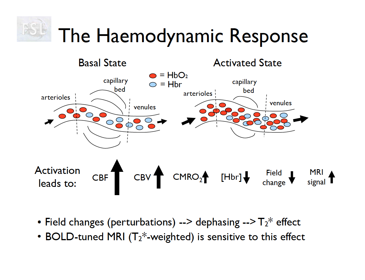
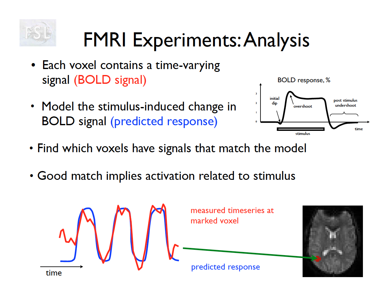
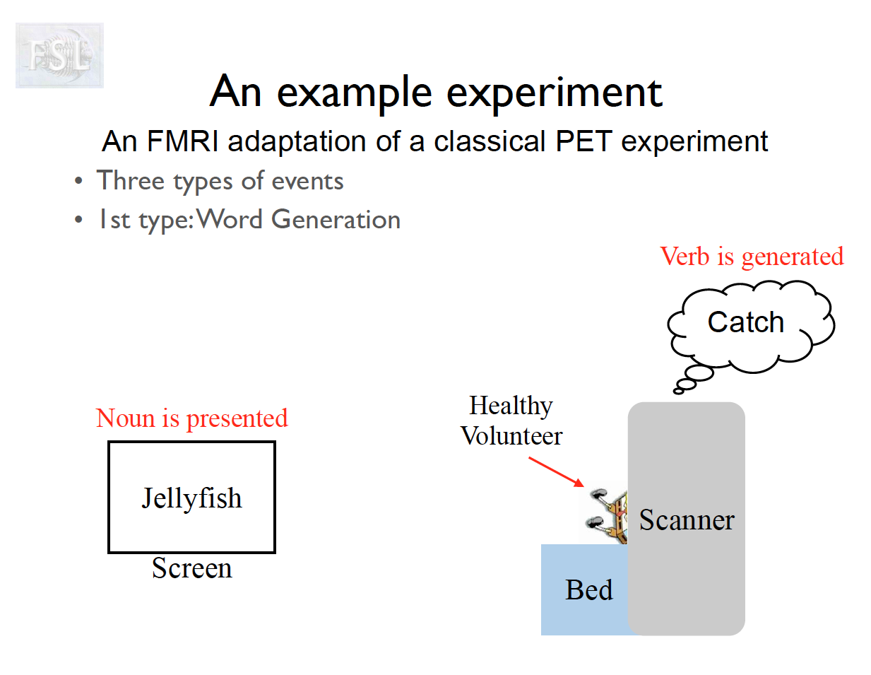
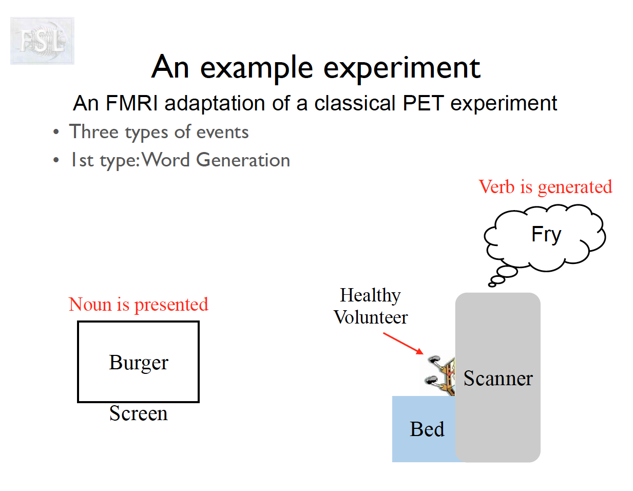
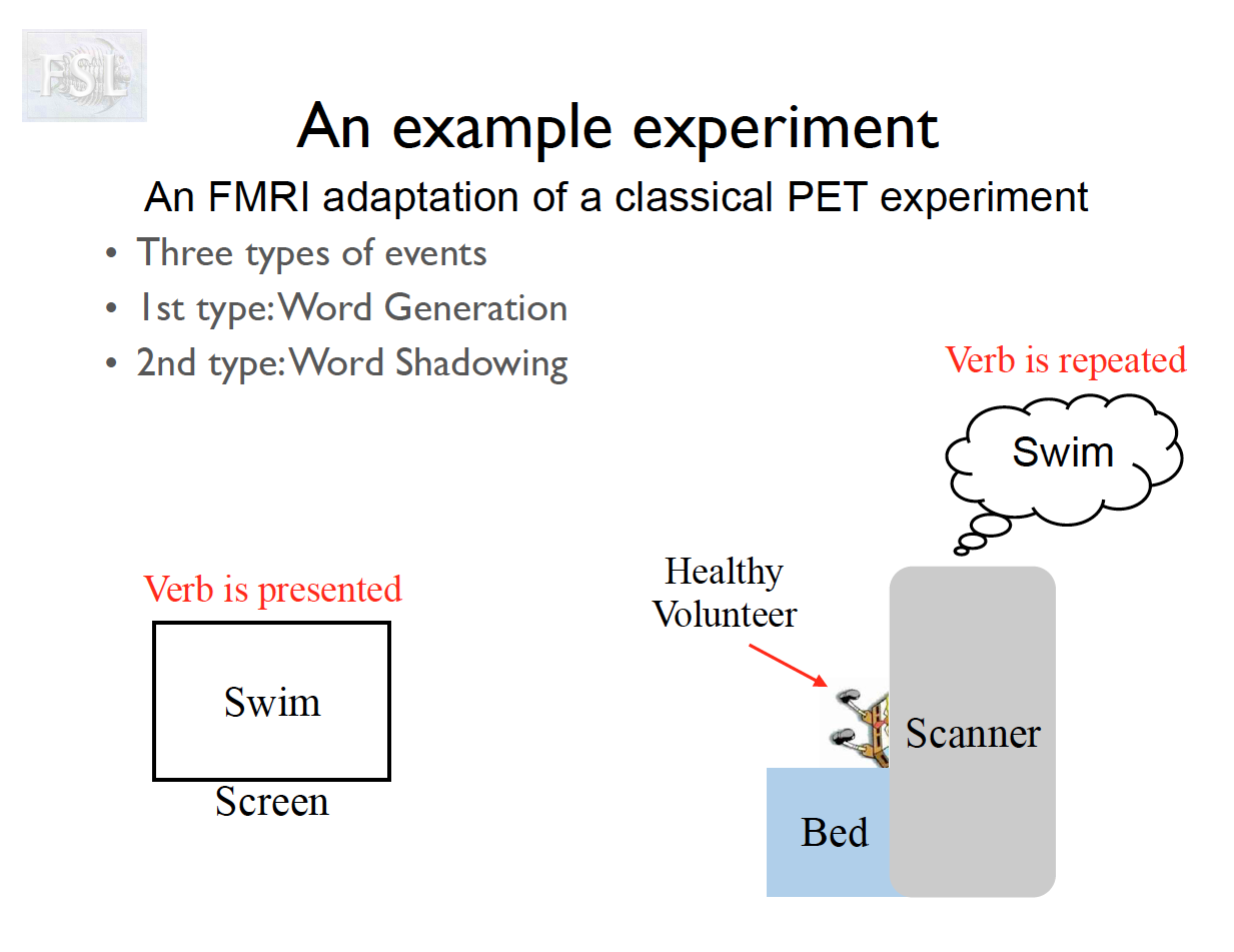
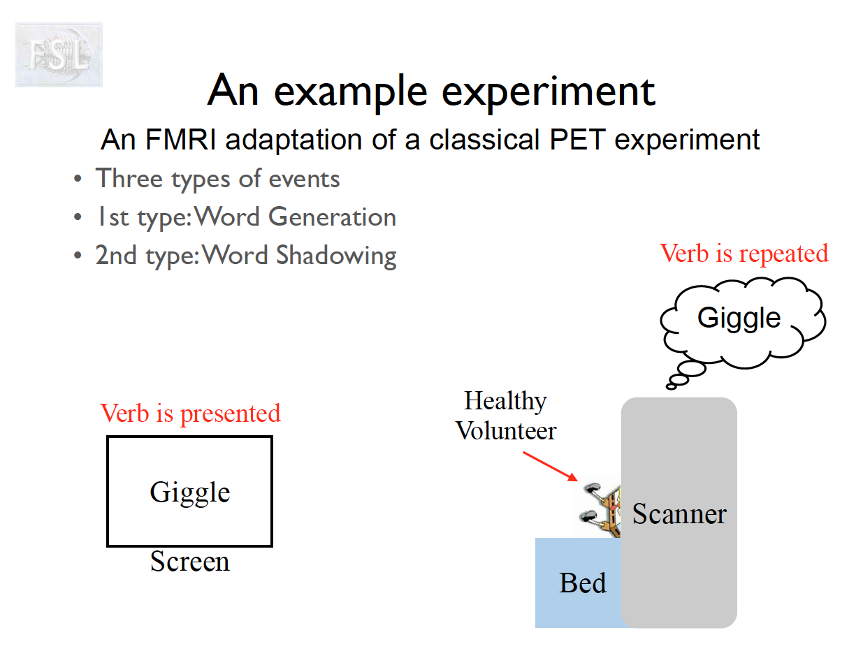
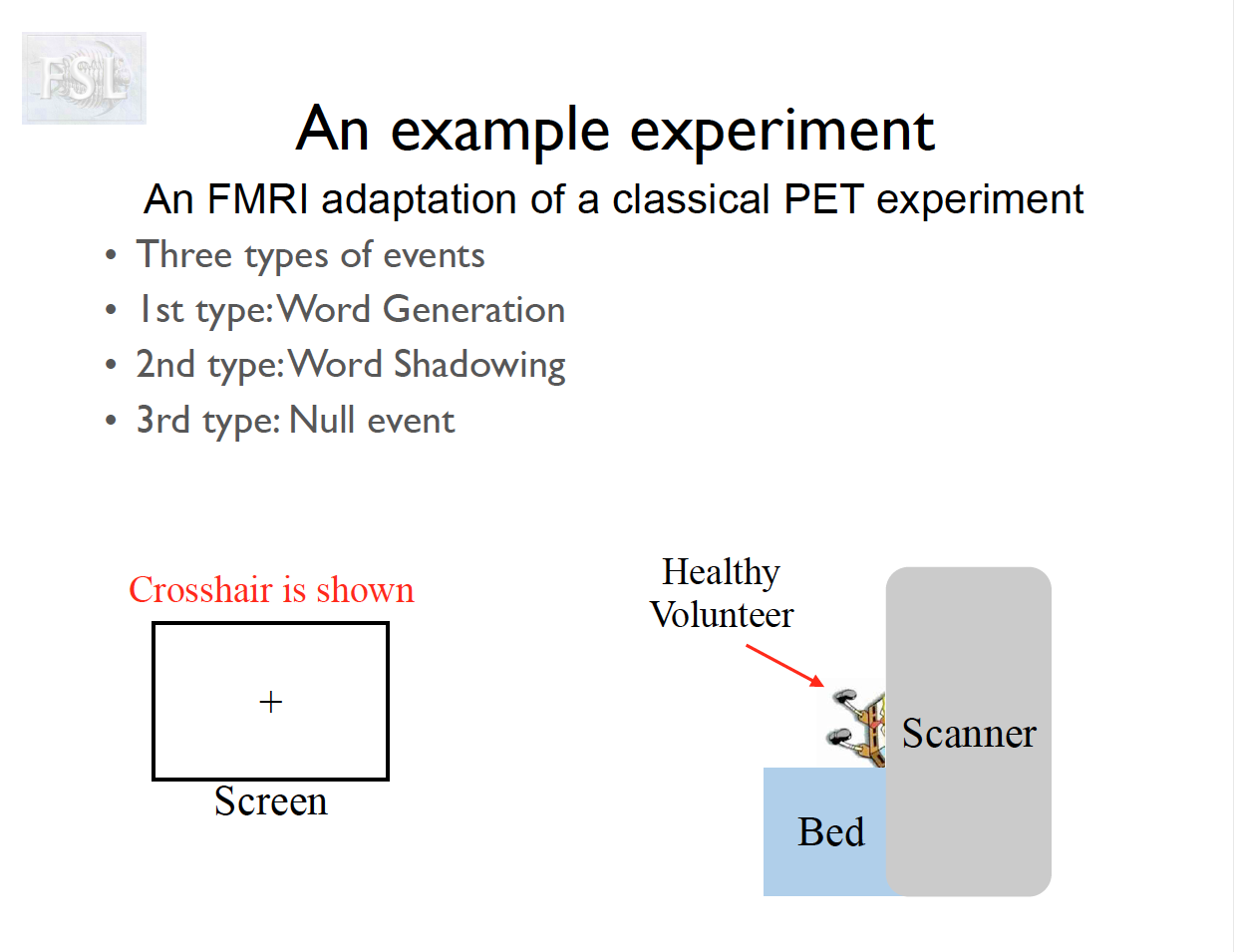
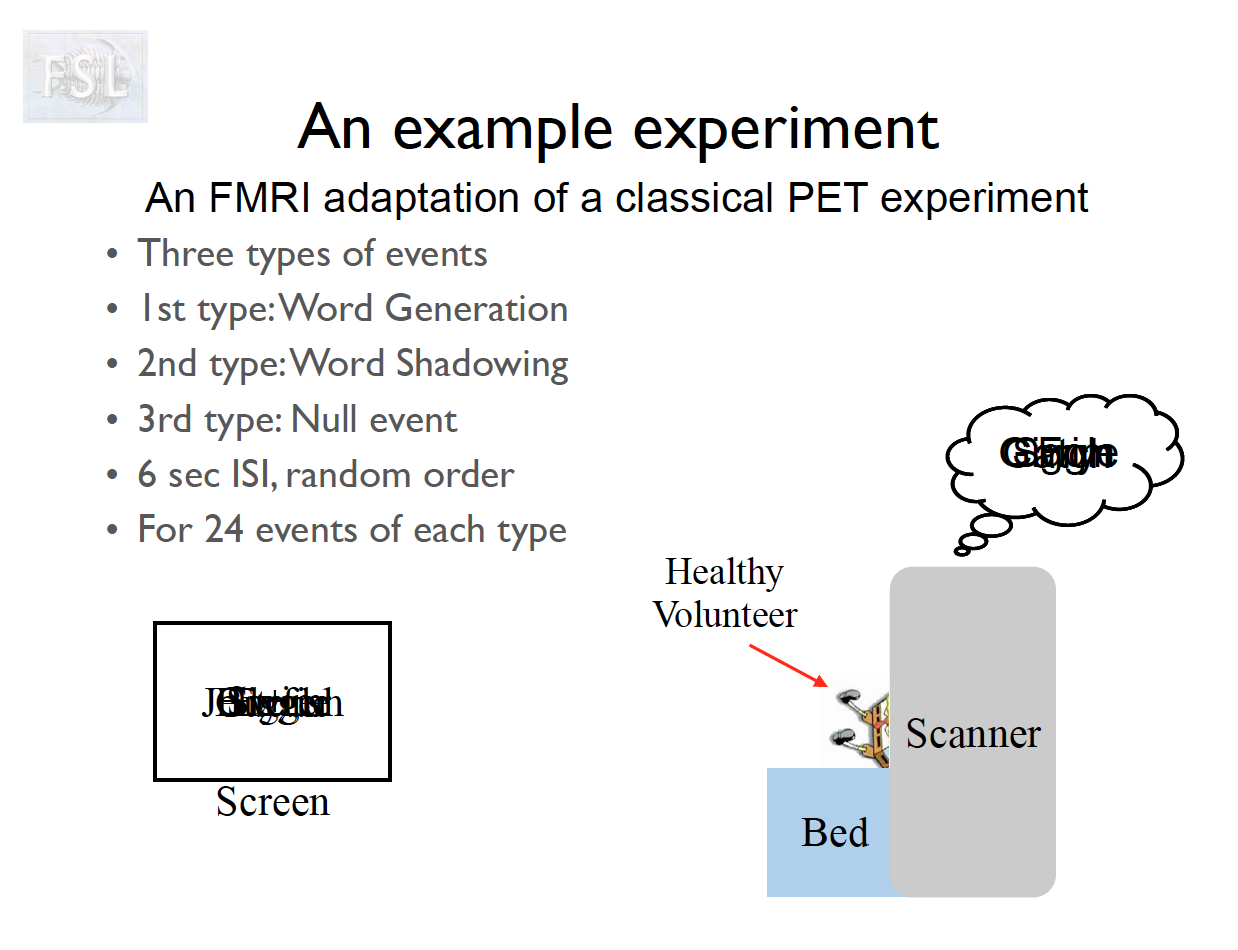
What is fMRI?

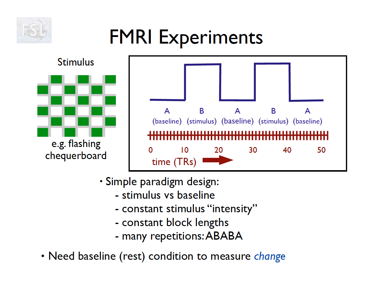
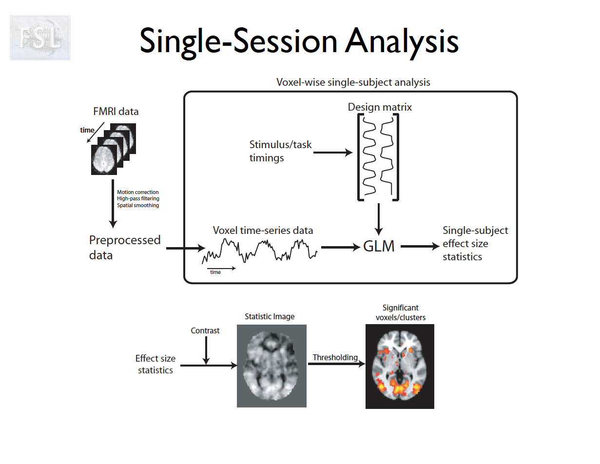
Basic task fMRI Analysis

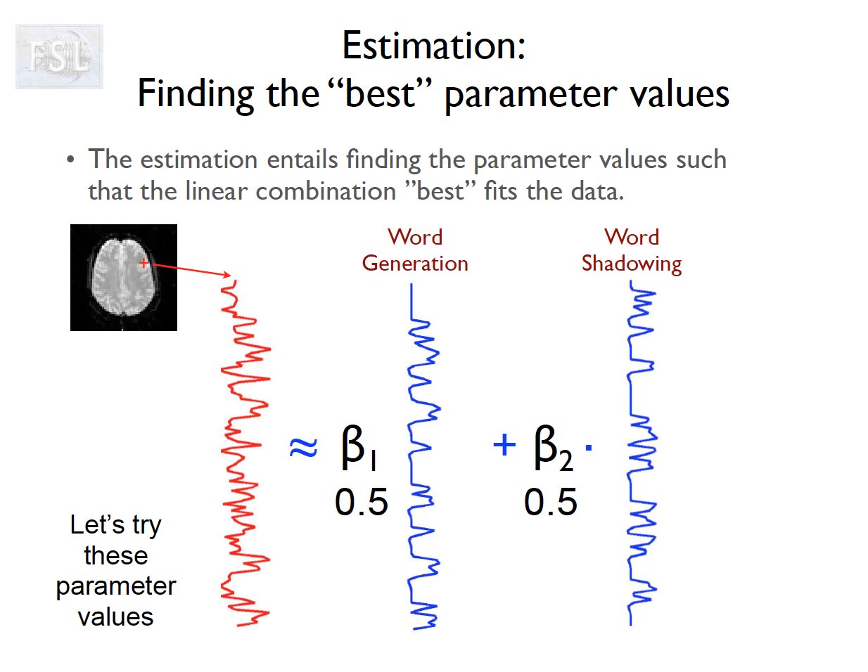
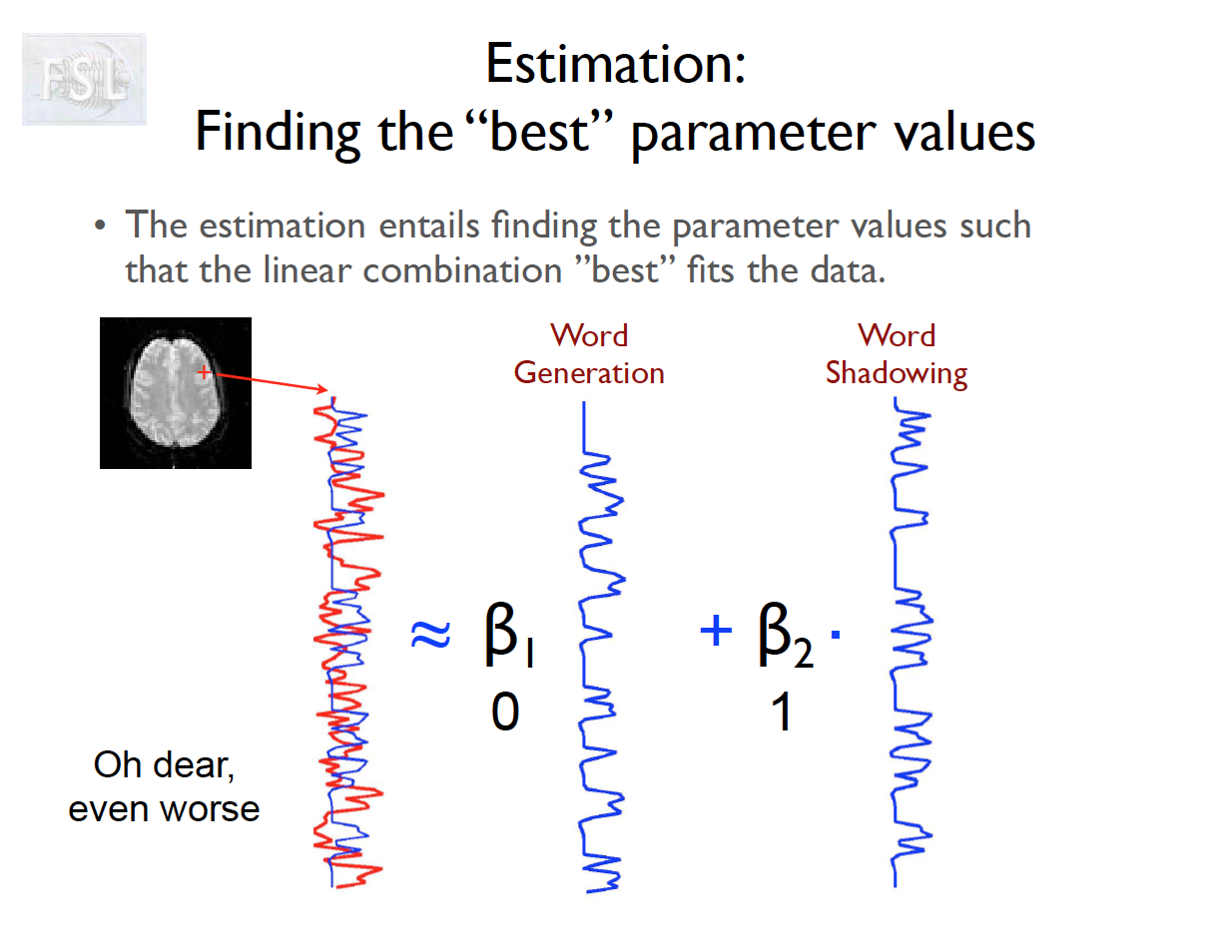
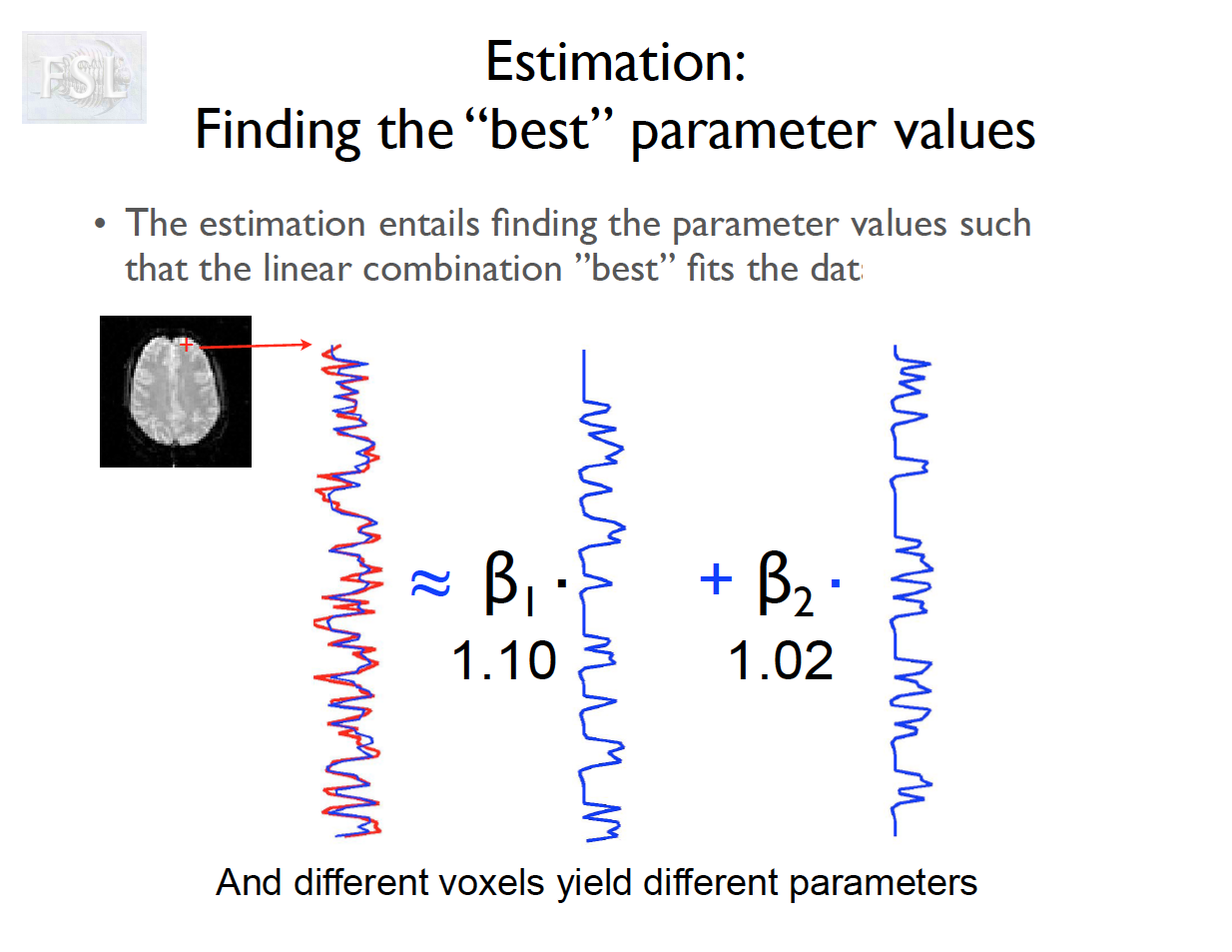
Important points

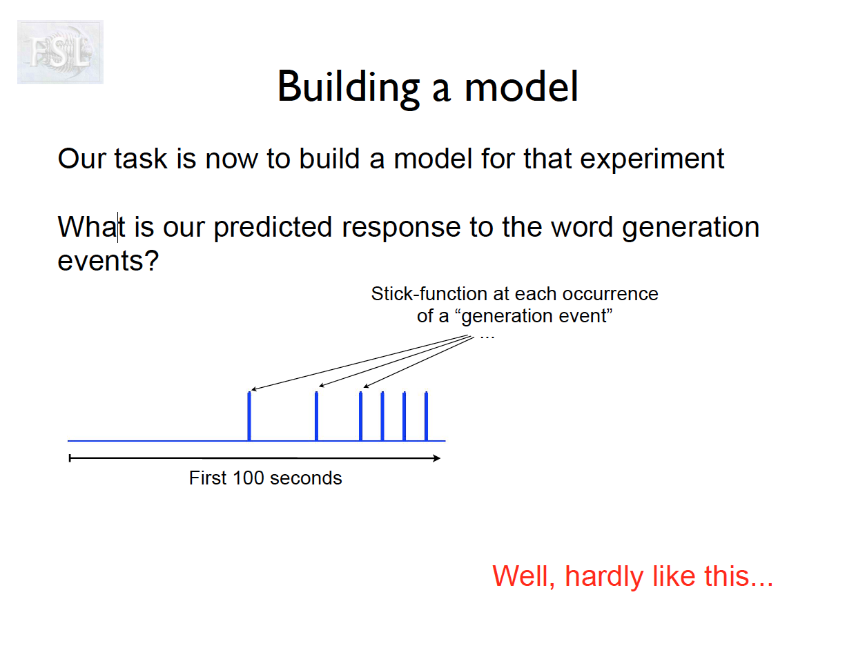
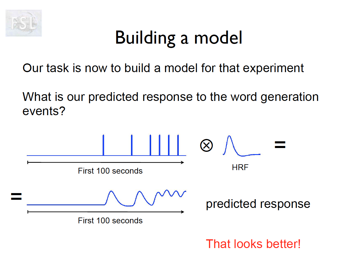
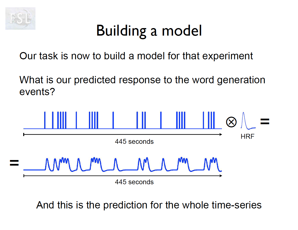
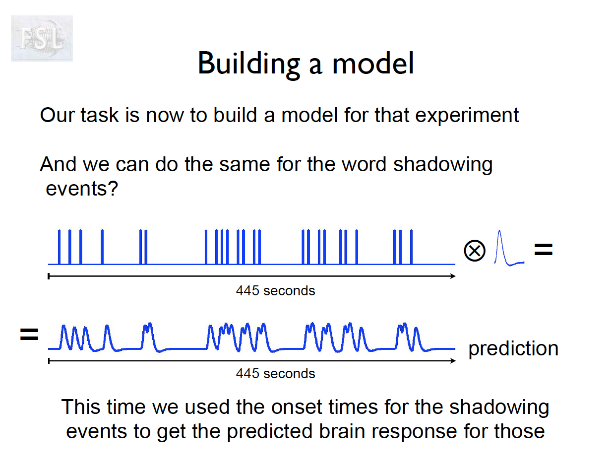
• task fMRI data independent variables (covariates) are determined by task stimulus series
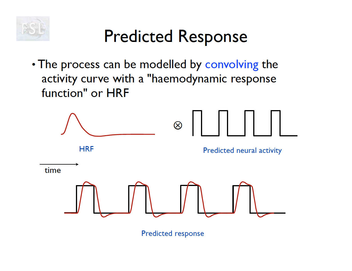
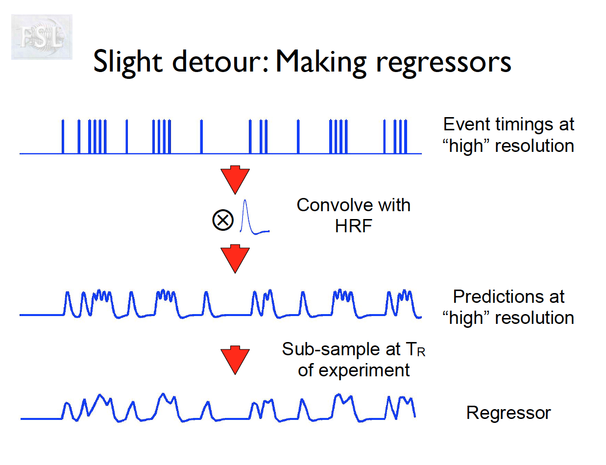
• And assume hemodynamic response function (double Gamma HRF)
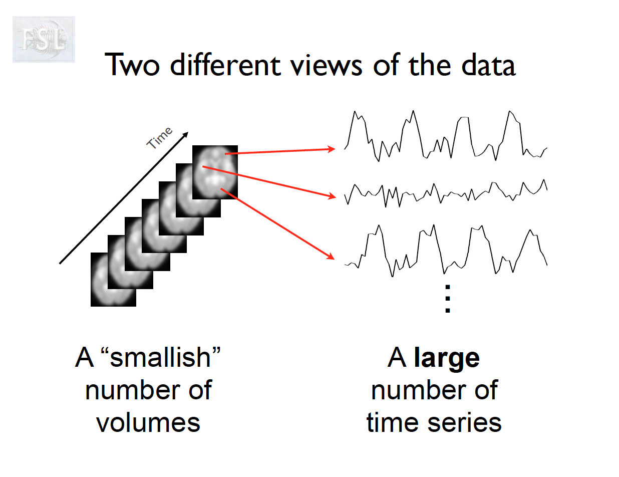
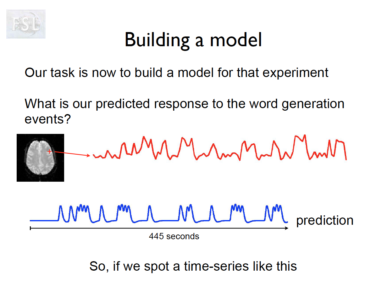
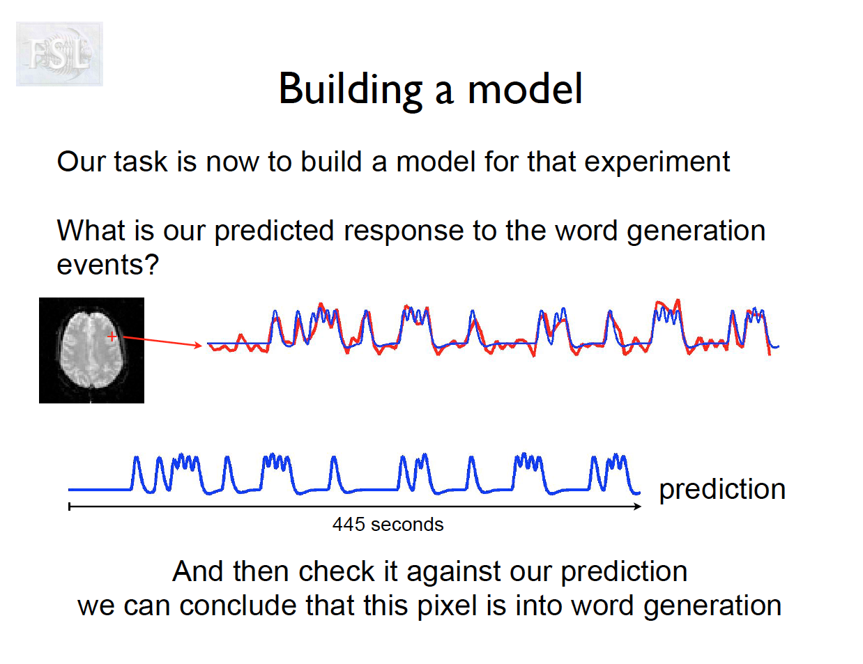
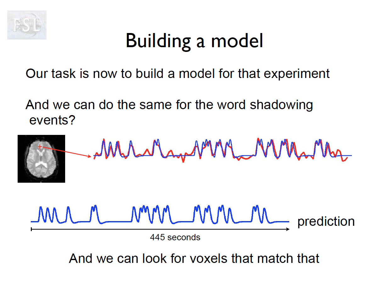
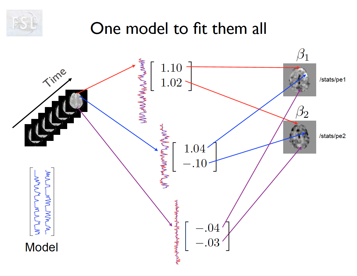
• Models are fit independently at each voxel (spatial location)
• We are only talking about fitting models for one participant, right now.

Time series analysis

Complications with time series

• fMRI time series analysis is more complex than described above
• What critical assumption is violated?
  • What will it affect in the model output?
  • Think bias and variance of \hat\beta and \hat\sigma_{\hat\beta}^2
• Univariate time series models (such as ARMA) require careful model fit evaluation that is impossible when fitting 150,000 models across the brain

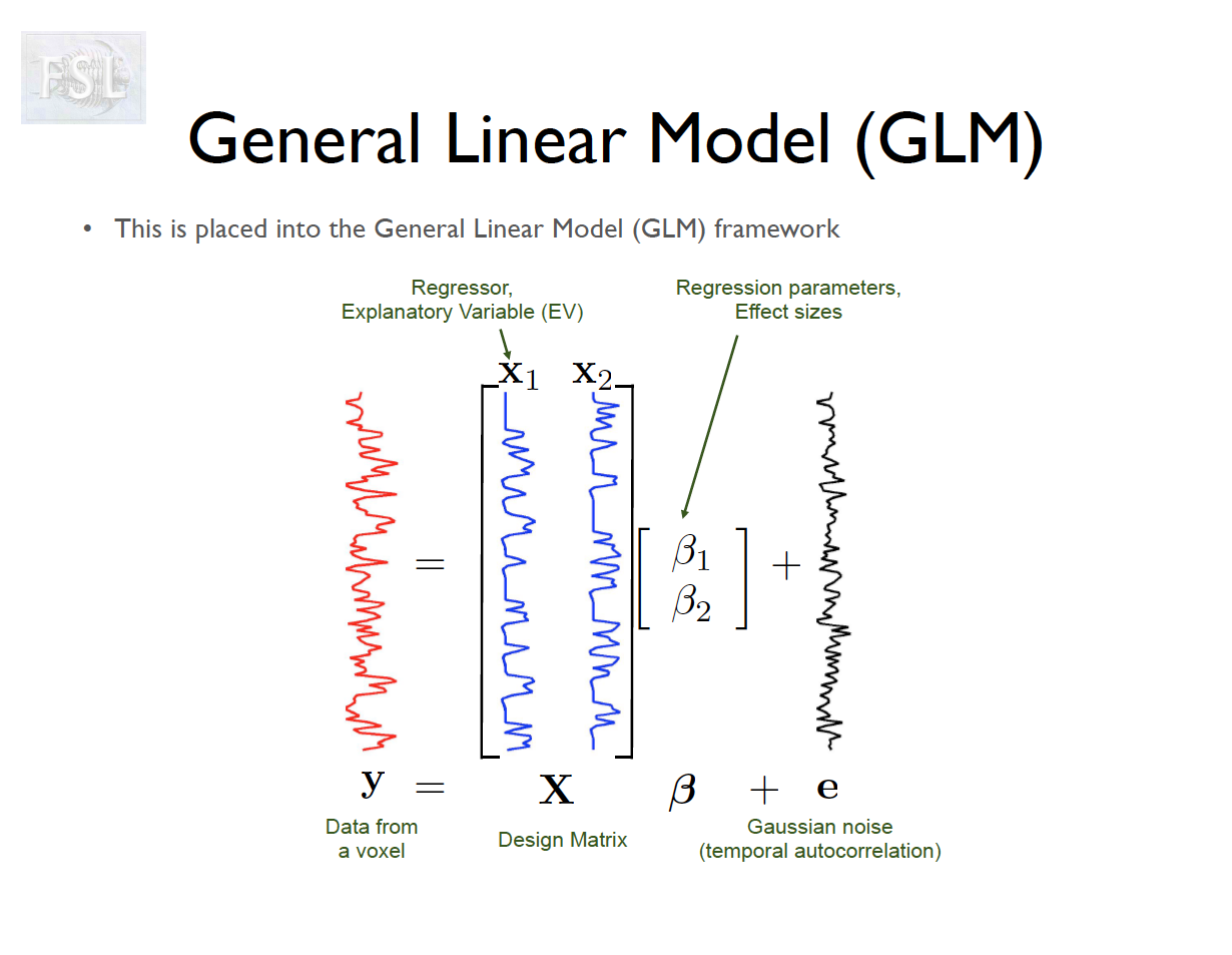
General linear models with prewhitening

• Notes here, based on FILM prewhitening
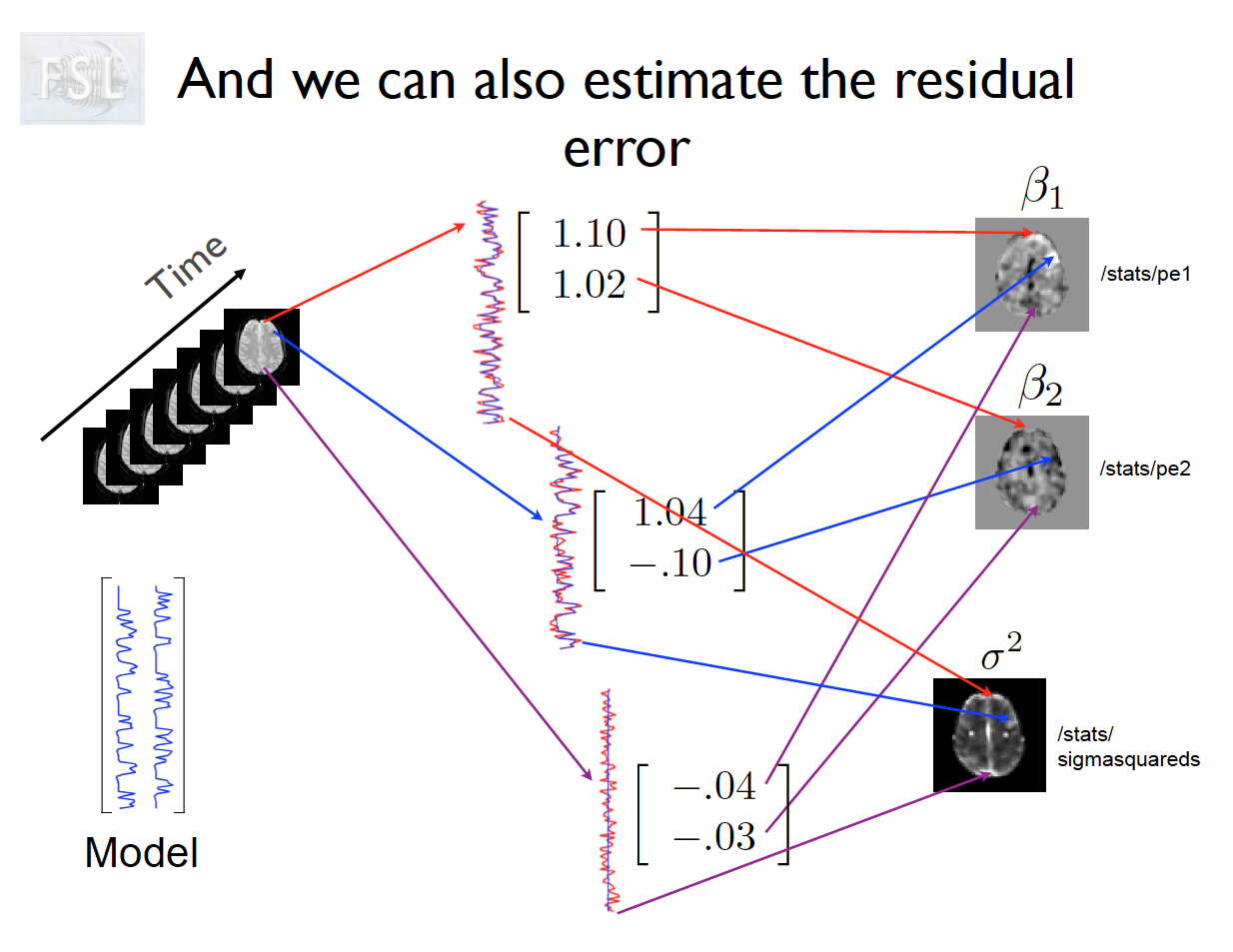
• For a single voxel v:

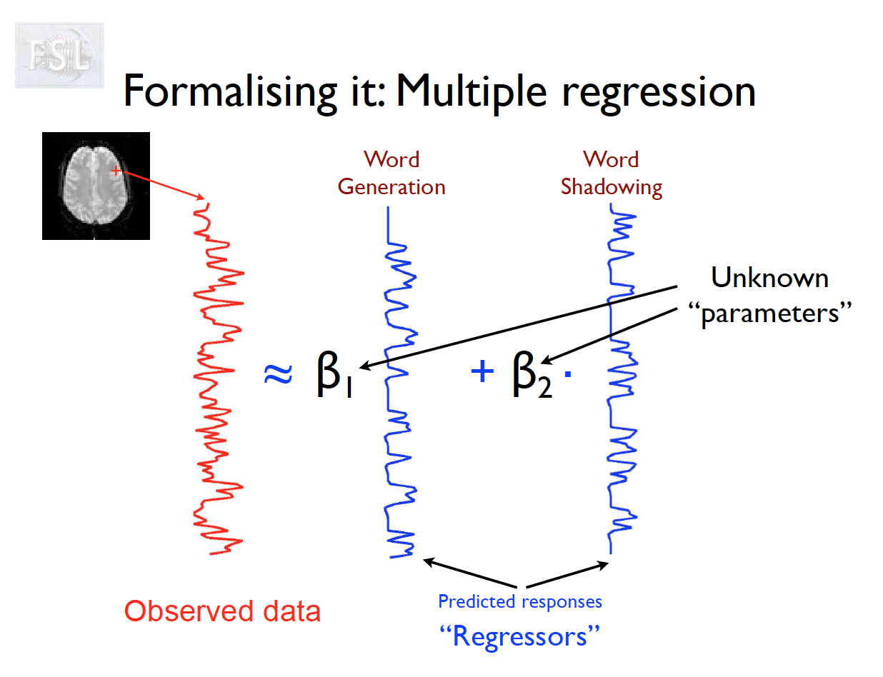
y(v) = X\beta(v) + \varepsilon(v)

• Can ignore v, since we are applying across all voxels separately
• X \in \mathbb{R}^{T \times p}: Design matrix (task regressors, confounds)
• \beta \in \mathbb{R}^p: Parameter vector
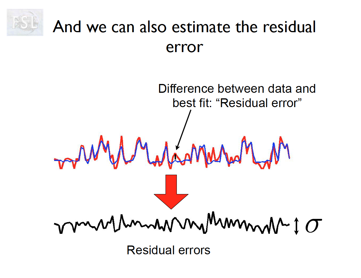
• \varepsilon \in \mathbb{R}^T: Error
• Assumptions: \mathbb{E}[\varepsilon] = 0, \mathrm{Cov}(\varepsilon ) = \sigma^2V (nonindependent errors)
• If V treated as proportional to the identity matrix, it will lead to inflated false positive rates (Woolrich et al., 2001)

Naive analysis:

What is the expected value of the least squares estimator? \mathbb{E}(\hat \beta) = What is the variance of the least squares estimator? \mathrm{Var}(\hat \beta) =

• A naive variance estimator \hat\sigma^2 (X^TX)^{-1} will be biased.
  • Standard errors and test statistics will be biased.
• What is a solution?

Prewhitening Concept

• Solution: transform model so residuals are uncorrelated

Given:

y = X\beta + \varepsilon, \quad \mathrm{Var}(\varepsilon) = \sigma^2V

Let K be a square root matrix of V such that:

K V K^T = I

• Apply K to both sides:

K y = K X \beta + K \varepsilon

• What is the marginal distribution of Ky?
• This is prewhitening: transforms correlated errors into “white noise”
• As you’ve seen, fMRI data are also high-pass filtered to remove low-frequency components.
  • The notation in the paper assumes this was already done, resulting in the covariance V
• New Problem: V and K are unknown and need to be estimated.

FILM Approach (Woolrich et al., 2001)

• FMRIB’s Improved Linear Model:
• One-step prewhitening to estimate V
• Many potential time series models to choose from
• FILM models autocorrelation with voxel-wise tapered estimates

Features of time series data

1. Auto-correlation
2. Frequency domain interpretation

Ways to estimate V

• For an arbitrary time series x(t) we can compute some estimators of the autocorrelation
• Raw estimator for correlation with lag \tau

r_{xx}(\tau) = \frac{1}{\hat\sigma^2} \sum_{t=1}^{N-\tau} x(t) x(t+\tau)/(N-\tau)

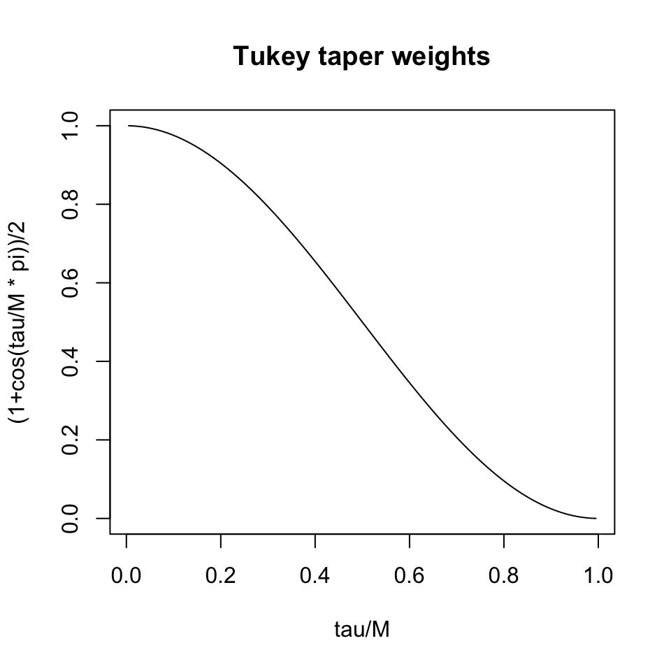
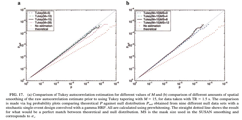
• Tapered estimators, such as the Tukey single-tapering

\hat\rho_{xx}(\tau) = \frac{1}{2}\left( 1 + \cos\left(\frac{\pi \tau}{M}\right) \right) r_{xx}(\tau)

for \tau<M and zero otherwise.

• Others not discussed here (see Woolrich et al., 2001)

• Matrix V can be filled in with these empirical estimators as a Toeplitz matrix

• If \beta is known, the formulas are computed with \epsilon = y - X\beta

• Alternatively, we could use \hat\beta, giving the residuals r = (I- X(X^T X)^{-1} X^T) y

• What is the autocorrelation of the residuals?

\mathrm{Cov}(r) =

• It is not quite V and V cannot be directly estimated from r. Woolridge et al suggested it is close enough.

Iterative procedure for prewhitening

• \hat\beta is not the BLUE when the covariance of \epsilon is V
• The BLUE is X^T V^{-1} X)^{-1} X^T V^{-1} y (not possible to compute this)
• After obtaining estimate for V (and or K), fit OLS:

\hat{\beta}_1 = (X^T \hat V^{-1} X)^{-1} X^T \hat V^{-1} y

• Then the we could compute a new \hat V and iterate until convergence.
• This would take ages across 150,000 voxels, so instead, they just recompute \hat \beta_1 once

Evaluation

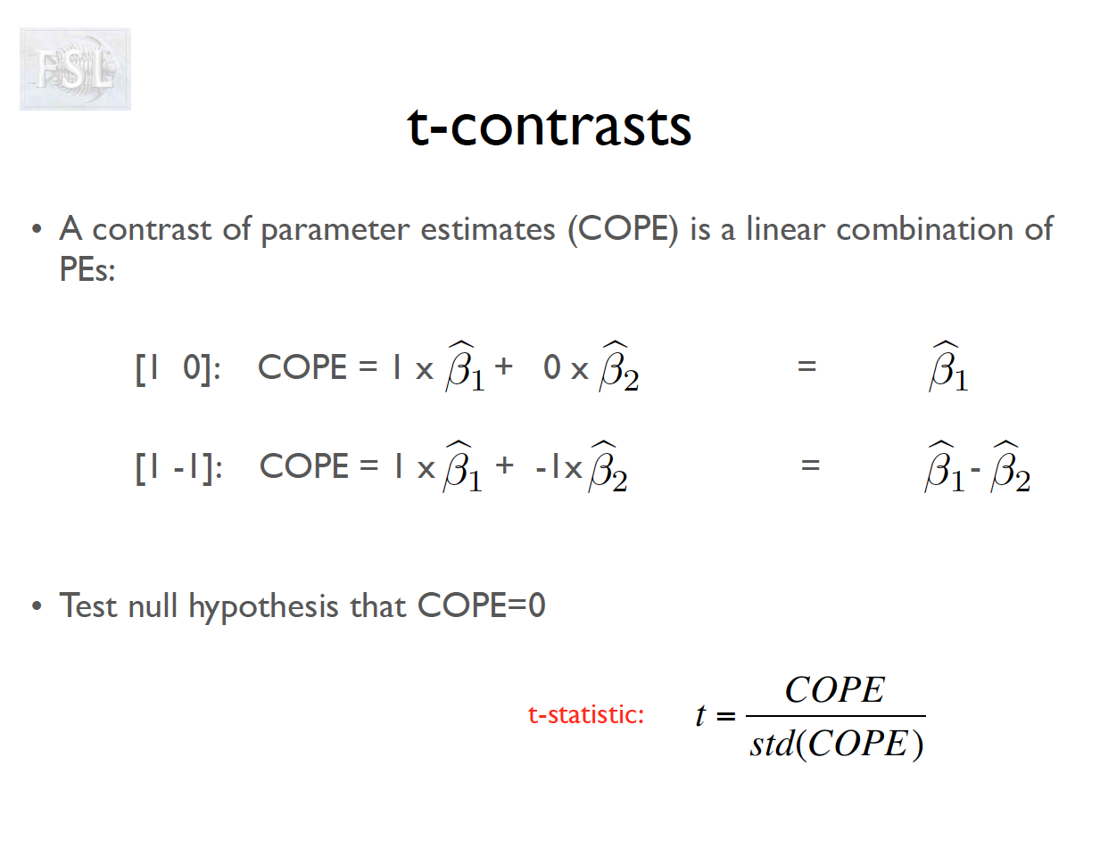
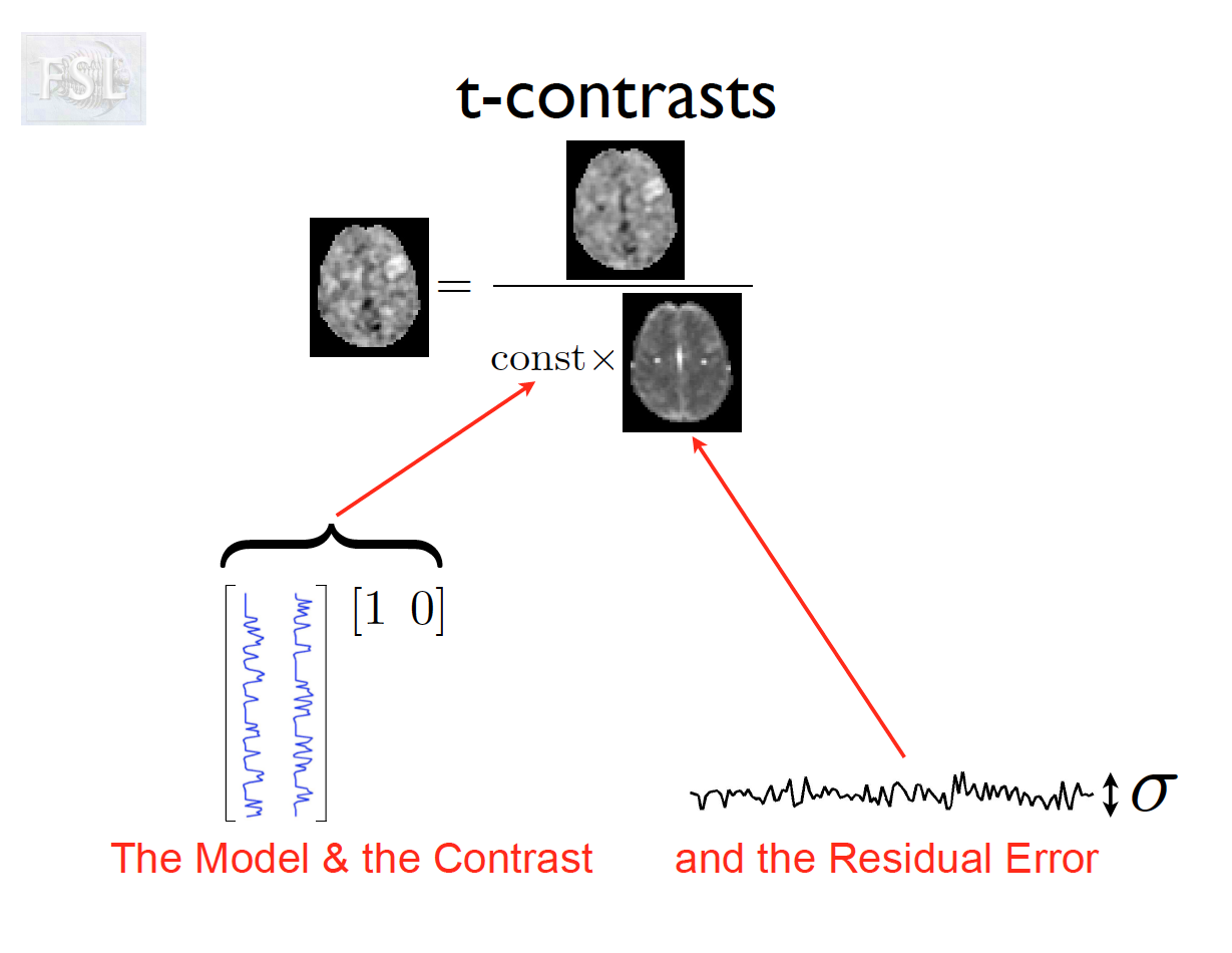
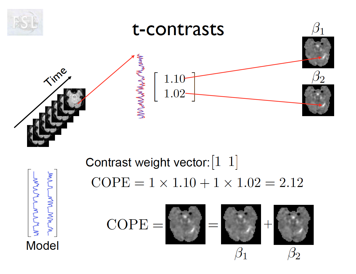
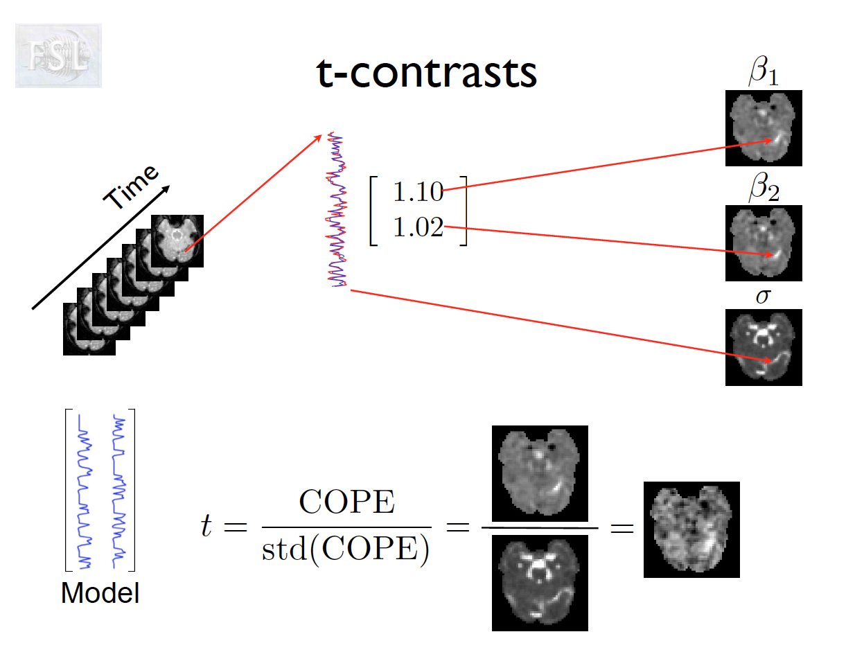
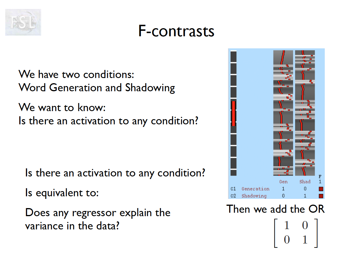
• Contrasts (T- and F-statistics) can be computed:

t = \frac{c^T \hat{\beta}}{\hat{\sigma} \sqrt{c^T (X^T \hat V^{-1} X)^{-1} c}}

and should be approximately normally distributed under the null, in large samples.

Tukey QQ plot with smoothing (MS)

References

• Woolrich MW, Ripley BD, Brady M, Smith SM. (2001) Temporal autocorrelation in univariate linear modeling of fMRI data. NeuroImage, 14(6):1370–1386.
• Friston KJ, et al. (1995) Statistical parametric maps in functional imaging: a general linear approach. Human Brain Mapping, 2(4):189–210.

Frequency domain transformations

• e.g. Fourier and Wavelet transformations
• Used a lot in imaging for spatial and temporal frequency domain transformations
• Processing and analysis in the frequency domain has a lot of advantages
• I won’t cover it here, as I’m not an expert, but we could come back to it

Despicable Me

• Interactive: we are going to finish first-level analyses of the Despicable Me dataset
• You will run batch processing on a subset of participants and do QA for the next assignment

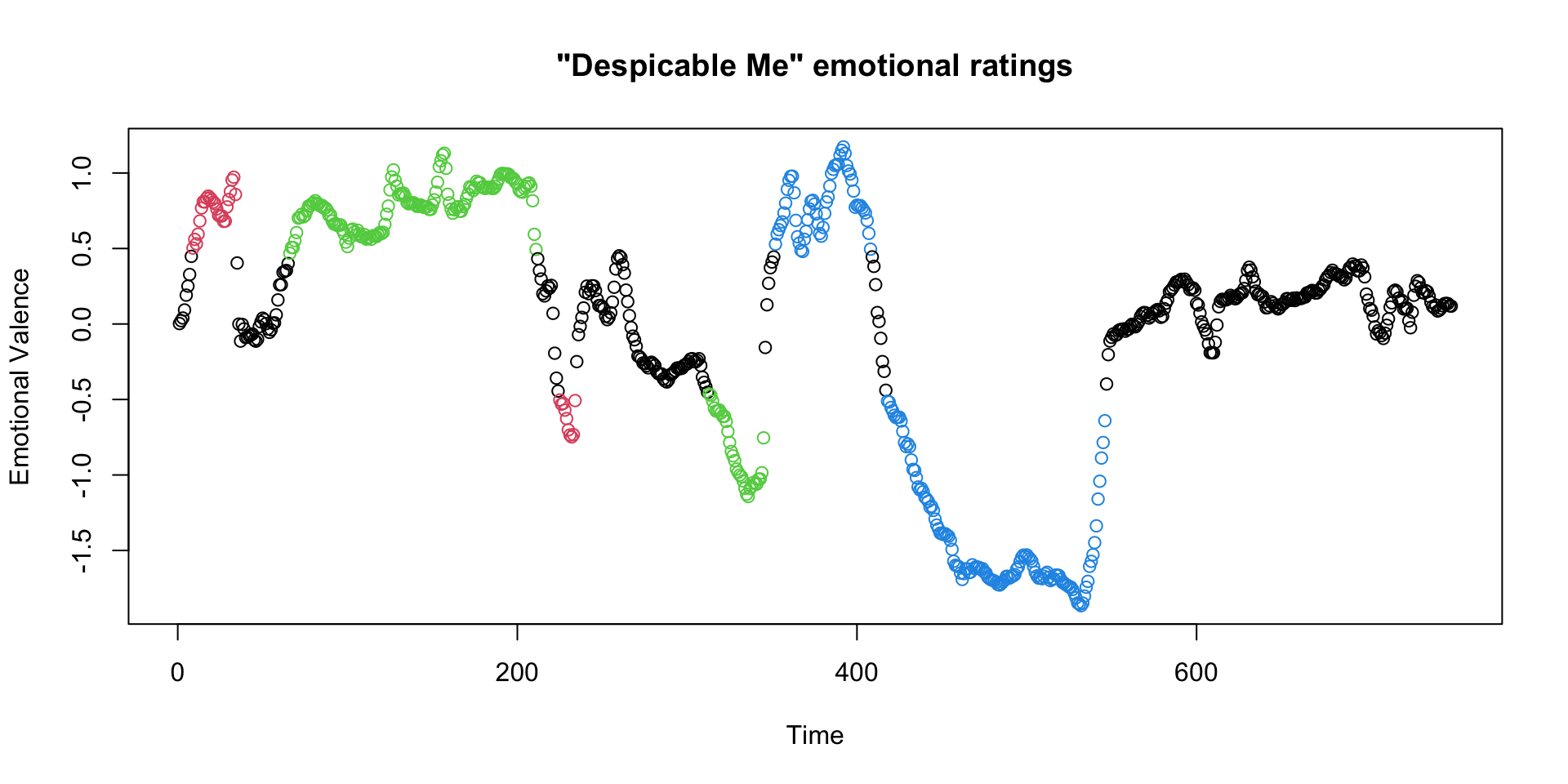
Naturalistic viewing task Despicable Me

• We will analyze Naturalistic viewing data
• Naturalistic viewing of Despicable Me (Furtado 2024)
• Despicable Me clip on Netflix 1:02:09 - 1:12:09

Despicable Me

Stimulus time series

• Naturalistic viewing task does not have strict “events” that occur during the task
• Some recent research created continuous emotional ratings for the Despicable Me clip
• We can use these to define particular “blocks” of particular emotional states during the clip

dm = readRDS('../data/RBC/stimulusTimeSeries/despicableMe/emotionBlocks.rds')
plot(dm$emo_valence, type='p', ylab='Emotional Valence', xlab='Time', main='"Despicable Me" emotional ratings',
     col=as.numeric(dm$positiveBlock) + as.numeric(dm$negativeBlock) -1)

Input into FSL FEAT GUI

• The code below creates a file with the stimulus time series needed for FSL’s FEAT GUI

# path to fsf file for preprocessing for first participant
# /Users/vandeks/Library/CloudStorage/Box-Box/SMN/data/RBC/HBN_BIDS/sub-NDARAA306NT2/ses-HBNsiteRU/func/sub-NDARAA306NT2_ses-HBNsiteRU_task-movieDM_bold.feat/design.fsf
TR = 0.8
pos = rle(dm$positive)
pos$lengths[1] = (pos$lengths[1] - 6)
# first one starts at zero
pos$starts = c(0, cumsum(pos$lengths)[-length(pos$lengths)]+1)
# output needed by FSL
threeCol = data.frame(onset=pos$starts*TR, duration=pos$lengths*TR, value=pos$values)
write.table(threeCol[threeCol$value==1,], row.name=FALSE, sep=' ', col.names = FALSE, file='../data/RBC/stimulusTimeSeries/despicableMe/positiveStimulus.txt')
# /Users/vandeks/Library/CloudStorage/Box-Box/SMN/data//RBC/stimulusTimeSeries/despicableMe/positiveStimulus.txt

• To input the stimulus time series into FSL, we provide a 3 column text file with the following info
  • Onset, Duration, Value
• Include temporal derivative and apply temporal filtering.

Create a similar stimulus time series for the negative emotional blocks

Design setup

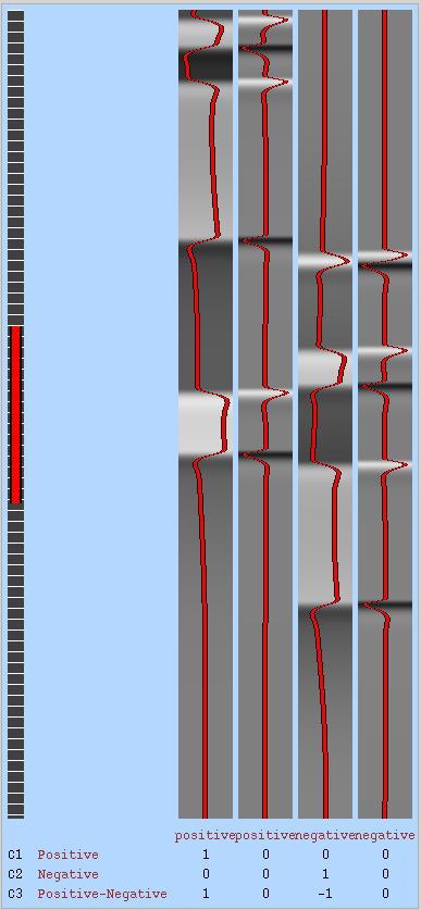
Design matrix

Assigning participants to students

• Sites have different scan parameters, which means we need to process the data differently for each site
• Here, we’ll assign each of you a chunk of participants to process from the same site
• (More on site harmonization later)

sites = read.table(file = '../data/RBC/sites.txt', sep = '/', header = FALSE, col.names=c('subject', 'site'))
table(sites$site)

resting state fMRI preprocessing

A lot of this preprocessing occurs in a regression framework

Recap of task fMRI processing

• Inhomogeneity correction
• Brain extraction (via structural image)
• Registration
• Motion correction
• Slice timing correction
• Distortion correction (if field map available)
• Temporal filtering & confound regression
• Spatial smoothing

rs-fMRI unique processing

• rs-fMRI is highly sensitive to motion artifact and noise
• More aggressive preprocessing steps:
  • Scrubbing – removing/modeling out high-motion time points
  • Intensive nuisance covariate removal (24 parameters)
  • Band-pass filtering (removing high frequency components as well)
  • Independent Components Analysis (ICA) denoising – potential alternative to regression

References Ciric et al., 2017 Parkes et al. 2018

Band-pass filtering

• Similar, but keeping only frequencies in a range
• Performed at the same time as nuisance regression

Nuisance regression (related to motion)

• Motion – 24 parameters total
  • Translation and rotation – 6 total parameters
  • Derivatives – 6 more
  • Squares of translation and rotations
  • Squares of derivatives

Nuisance regression (nuisance signal)

aCompCor – Anatomical Component Correlation

• In addition to motion covariates
• CSF and white matter are not “active” – regress out signal associated with these
• PCA of the signal in these regions, e.g. Y_{\mathrm{CSF}} \in \mathbb{R}^{T \times V_{\mathrm{CSF} }} \\ Y_{\mathrm{CSF}} = U D W^T Choose the first K components and regress them out of the data

Global signal regression

• Controversial because there is evidence it increases motion-related correlations between distant brain regions
• I am not too familiar why, could be a good advanced topic
• REFs.

Scrubbing

“Dummy”/“One hot” coding of scans where participant move a lot

In the end, the preprocessing regression design matrix for rs-fMRI might look something like

\begin{bmatrix} \vert & \vert & \vert& \vert \\ \text{Temp filt} & \text{Motion} & \text{aCompCor} & \text{Dummy variables} \\ \vert & \vert & \vert & \vert \end{bmatrix}

rs-fMRI before and after preprocessing

• Histogram of signal changes
• Positive/negative correlations are relative to preprocessing

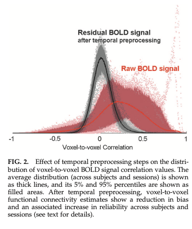
Whitfield-Gabrieli 2012

rs-fMRI first-level analysis

• Pretty straightforward after preprocessing
• Functional connectivity is defined as Pearson correlation between two locations (R(v,t) is the residuals from the preprocessing)

\hat \rho(v,w) = \frac{\sum_{t=1}^T R(v, t) R(w, t)}{\sqrt{\sum_{t=1}^T R(v, t) ^2 \times \sum_{t=1}^T R(w, t)^2 } } * Correlations are Fisher Z-transformed so that they are approximately normal

Z(v,w) = \mathrm{atanh}(\hat \rho(v,w))

• Types of analyses
  • Network – all voxel-to-voxel or region-to-region correlations
  • Seed-based – Correlation of preselected seed region with entire image (image-valued)

Overview of rs-fMRI

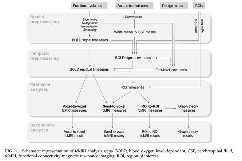
Whitfield-Gabrieli 2012