Class 2

Author

Simon Vandekar

Objectives:

Learn some basic concepts about probabilities
Learn to use probability to think about data
But first, we will recap some statistica jargon and practice using it to describe the data.

Some common statistical jargon so far

Types of variables

Categorical variable - a variable that takes discrete values, such as diagnosis, sex,
Continuous variable - a variable that can take any values within a range, such as age, blood pressure, brain volume.
Ordinal variable - a categorical variable that can be ordered, such as age category, Likert scales, Number of days, Number of occurrences.

Distribution/Density features

Mode/ Non-modal/Unimodal/ Bimodal - a peak in a density.
- Non-modal - no peak
- Unimodal - one peak
- Bimodal - two peaks
Quantile - the pth quantile, q_p divides the distribution such that p% of the data are below q_p.
- Median - 50th quantile of a distribution
Skew/Skewness - the amount of asymmetry of a distribution
- Symmetric distribution - a distribution with no skew
Kurtosis - the heavy tailed-ness of a distribution.

Bivariate distribution features

Correlation/correlated - two variables are linearly dependent
Dependent - two or more variables are related to each other in some way
Independent - two variables that are not related to each other

Practice (15 min)

Below are some questions related to some of the material we’ve covered so far. We’ll look at an insurance dataset with the amount of charges as a function of health and demographic features.

Insurance companies are often interested in predicting charges so that they can know who high-risk individuals are based on easily measurable demographic information.

For each of the variables in the table below describe which are continuous, ordinal, or categorical. They might be one or more of these things.
- Age -
- Sex -
- BMI (body mass index) -
- Children -
- Smoker -
- Region -
- Charges -

Code

library(RESI)

Registered S3 method overwritten by 'clubSandwich':
  method    from    
  bread.mlm sandwich

Code

library(reactable)
reactable(insurance)

The table below summarizes the variables in the dataset for nonsmokers smokers. For each of the variables in the table below, comment on the skewness and whether the variables look similar or different between smokers and nonsmokers.

Code

insurance$smoker = factor(insurance$smoker, labels = c('Nonsmoker', 'Smoker'))
label(insurance$smoker) = 'Smoking Status'
table1(~ age + bmi + children + sex + region + charges | smoker, data=insurance)

	Nonsmoker (N=1064)	Smoker (N=274)	Overall (N=1338)
age
Mean (SD)	39.4 (14.1)	38.5 (13.9)	39.2 (14.0)
Median [Min, Max]	40.0 [18.0, 64.0]	38.0 [18.0, 64.0]	39.0 [18.0, 64.0]
bmi
Mean (SD)	30.7 (6.04)	30.7 (6.32)	30.7 (6.10)
Median [Min, Max]	30.4 [16.0, 53.1]	30.4 [17.2, 52.6]	30.4 [16.0, 53.1]
children
Mean (SD)	1.09 (1.22)	1.11 (1.16)	1.09 (1.21)
Median [Min, Max]	1.00 [0, 5.00]	1.00 [0, 5.00]	1.00 [0, 5.00]
sex
female	547 (51.4%)	115 (42.0%)	662 (49.5%)
male	517 (48.6%)	159 (58.0%)	676 (50.5%)
region
northeast	257 (24.2%)	67 (24.5%)	324 (24.2%)
northwest	267 (25.1%)	58 (21.2%)	325 (24.3%)
southeast	273 (25.7%)	91 (33.2%)	364 (27.2%)
southwest	267 (25.1%)	58 (21.2%)	325 (24.3%)
charges
Mean (SD)	8430 (5990)	32100 (11500)	13300 (12100)
Median [Min, Max]	7350 [1120, 36900]	34500 [12800, 63800]	9380 [1120, 63800]

The plots below summarize each of the variables separately using histograms with densities.

For each of the histograms below comment on:
- Symmetry
- Skewness
- Mode(s)

Code

par(mfrow=c(2,2))
invisible(sapply(names(insurance)[sapply(insurance, is.numeric)], function(name){ hist(insurance[,name], xlab=name, main=name, freq=FALSE); lines(density(insurance[,name], adjust=1.5), lwd = 2) } ))

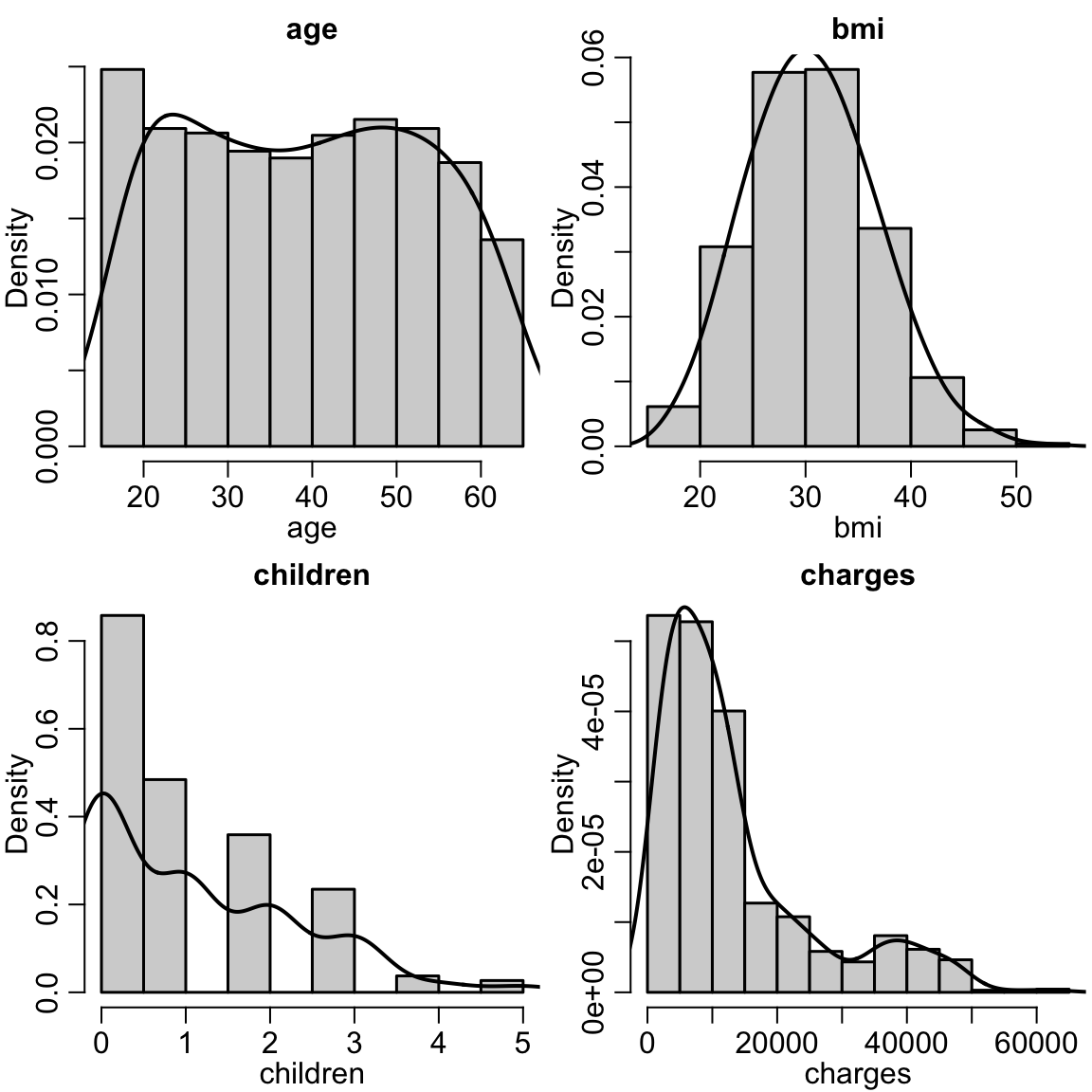
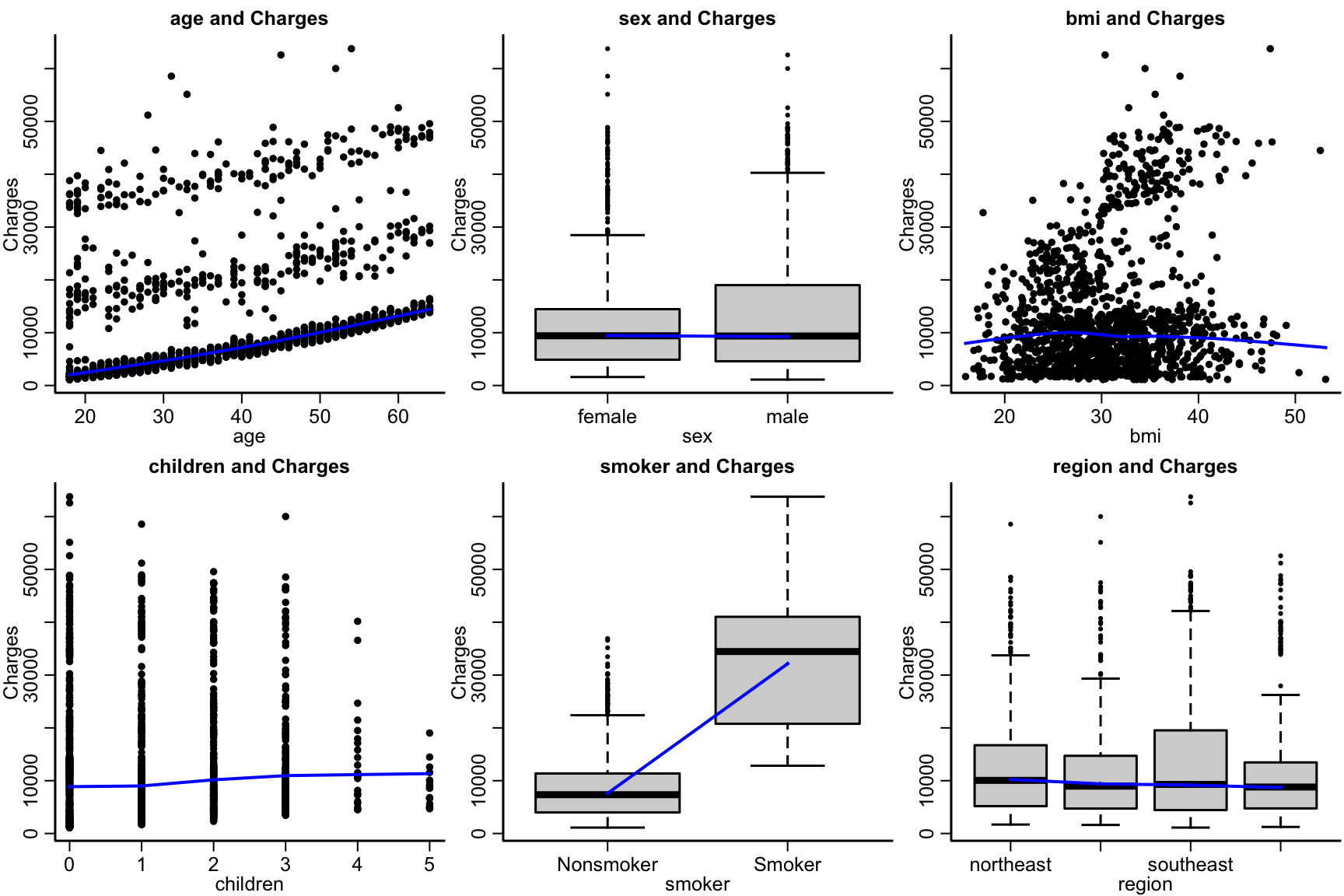
For each of the plots comment on the correlation and dependence of the variables with the number of charges.

Code

par(mfrow=c(2,3))
xvars = names(insurance)[1:6]
insurance$sex = factor(insurance$sex)
insurance$region = factor(insurance$region)
invisible(sapply(xvars, function(xvar){
  if(!is.factor(xvar)){
  plot(insurance[,xvar], insurance$charges, ylab='Charges', xlab=xvar, main=paste(xvar, 'and', 'Charges') )
  # remove missing values for lowess fit
  subset = na.omit(insurance[, c(xvar, 'charges')])
  lines(lowess( subset[,xvar], subset$charges), col='blue', lwd=2)
  } else {
   barplot(as.formula(paste('charges ~', xvar)), data=insurance)
  }
}))

Practice with plotting

It looks like for some of the plots above, there are multiple modes or clusters. Which ones? What could be driving these different clusters?
Create a scatter plot coloring the points for age and charges and BMI and charges by smoking status, to see if smokers fall in a particular cluster.

Why probability

Probability is the language of statistics.
It is how we can understand data and evaluate the quantitative methods we use.

Important tools in probability

Dependence/Independence Discrete random variables Continuous random variables Expected values/Averages CDF, PDF

Coin flips and diagnoses

Something that takes only two values can be described with a Bernoulli random variable.
- yes/no categories, e.g. smoking
- Diagnosis: schizophrenia or not, COVID+ or not

Bernoulli values x	probabilities
0 (nonsmoker)	1-p
1 (smoker)	p

What is a sensible value for p for the different Bernoulli variables above?

Random variables and probability notation

For X\sim \text{Be}(p): X is distributed as (\sim means “is distributed as”) Bernoulli, with parameter p \in (0,1), e.g. p=0.25.
Blackboard or capital P is probability, \mathbb{P}(X=x), means the probability the random variable X is equal to the nonrandom value x.
\mathbb{P}(X = x) = p^x(1-p)^{(1-x)}. That is the probability mass function (PMF) of a Bernoulli random variable
Common notation is f_X(x) is the PMF of the random variable X. In this case f_X(x):=p^x(1-p)^{(1-x)}.
:= notation means “is defined by.”
A random variable does not have a value in itself… We don’t usually talk about X=0.5, but \mathbb{P}(X=0.5).

Some questions:

For X\sim \text{Be}(p), what is the probability that X is 100?
What is the probability X is 0.5?
What is the probability X is 0?

Random sample to estimate smoking proportion

Let’s say the smoking status of each person in the insurance dataset is a random sample from X_i \sim \text{Be}(p), for i=1, \ldots, 1338.
What is a reasonable value for p?
How can we estimate what p is?

Multiple groups, Multinomial distribution

The multinomial can be used for distributions with multiple categories.
- Die rolls, Wordle number of guesses
- Likert scales (e.g. PANSS in schizophrenia), Tanner staging (puberty; 1-5), Cancer staging (0-4)
Number of children.
Region.
Let’s fill in this table together

y=Number of children	\mathbb{P}(Y=y)
0	___
1	___
2	___
3	___
4	___
5	___
6+	___??

What is the probability someone in the US has more than 5 children?
What is the estimated probability someone in the US has more than 5 children?
Write out the table for region and estimate the probabilities from the dataset.

Probability density function (PDF)

The probability density function f_X(x) for a random variable X can be thought of as \mathbb{P}(X=x).
It is called the probability mass function (PMF) for discrete random variables.

Number of children probability density function (PDF)

Let’s draw the estimated PDF for smoking status.
Let’s draw the estimated PDF for the number of children.
Let’s draw the estimated PDF for region.

Body mass index

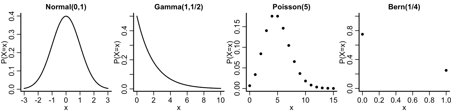
From the insurance dataset

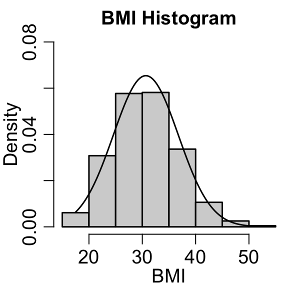
BMI is a continuous random variable, \mathrm{BMI} = \mathrm{weight}/\mathrm{height}^2
Here’s a plot from the insurance dataset.
It looks approximately normally distributed (not quite).
I’ve drawn the normal density on top

Code

library(RESI)
lims = hist(insurance$bmi, freq = FALSE, ylim=c(0, .08), main='BMI Histogram', xlab='BMI')
x = seq(min(lims$mids), max(lims$mids), length.out=100)
lines(x, dnorm(x, mean = mean(insurance$bmi),sd=sd(insurance$bmi)))