Class 3

Author

Simon Vandekar

Objectives:

  1. Learn some more basic concepts about probabilities
  2. Learn to use probability to think about data

Recap

  • We talked about PMFs and PDFs.

PDFs

Body mass index

From the insurance dataset

  • BMI is a continuous random variable, \mathrm{BMI} = \mathrm{weight}/\mathrm{height}^2

  • Here’s a plot from the insurance dataset.

  • It looks approximately normally distributed (not quite).

  • I’ve drawn the normal density on top

Code
library(RESI)
Registered S3 method overwritten by 'clubSandwich':
  method    from    
  bread.mlm sandwich
Code
lims = hist(insurance$bmi, freq = FALSE, ylim=c(0, .08), main='BMI Histogram', xlab='BMI')
x = seq(min(lims$mids), max(lims$mids), length.out=100)
lines(x, dnorm(x, mean = mean(insurance$bmi),sd=sd(insurance$bmi)))
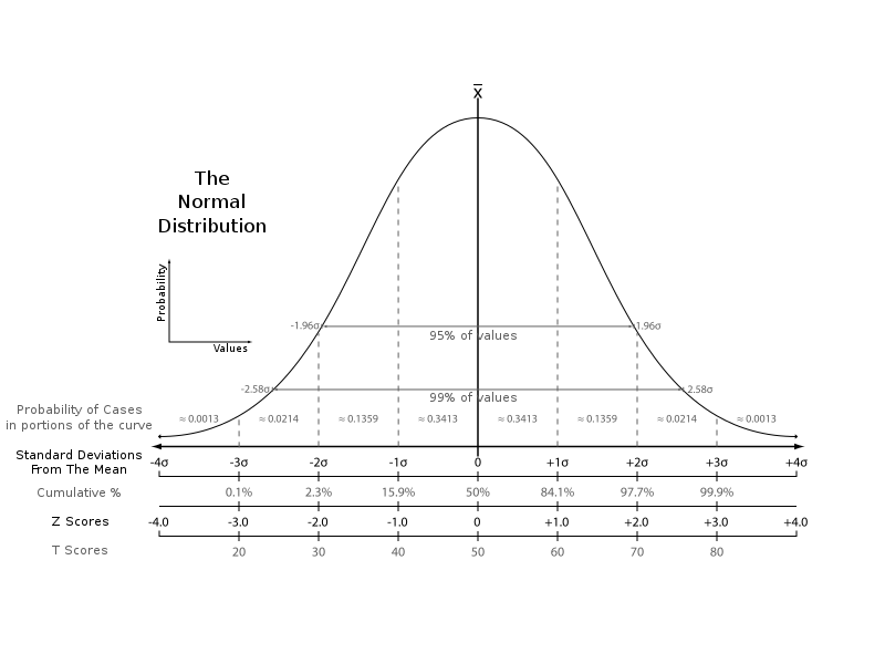
  • The normal distribution is f_X(x) = \frac{1}{2\pi \sigma^2} e^{-\frac{1}{2\sigma^2} (x - \mu)^2}

  • This is a picture of the standard normal distribution (\mu=0, \sigma^2=1).

  • In our dataset the mean is \hat \mu = 30.66, and the standard deviation is \hat\sigma = 6.1.
  • We can use f_X(x) to compute probabilities that a person’s BMI lies in a particular range.
    • Probability less than or equal to “healthy” – \mathbb{P}(X \le 25) = \int^{25}_0 f_X(x)dx
    • Probability in “healthy range” – \mathbb{P}(18 < X \le 25) = \int^{25}_{18} f_X(x)dx
  • The normal distribution is just an approximation.
    • Normal distribution is defined from (-\infty, \infty)

Cumulative Distribution Function (CDF)

The cumulative distribution function (CDF), F_X(x), for a random variable X is defined as F_X(x) = \mathbb{P}(X \le x). Here are some examples.

Some distribution functions.
  • What are some features that you recognize about these distribution functions?

For discrete random variables the derivative of the CDF does not exist because it is a step function, but the probability mass function is the amount the CDF jumps up at that location, heuristically we can define it as f(x) = F(x+\Delta x) - F(x), for an infinitesimal value \Delta x.

BMI example continued

  • CDF can be thought of as a percentile function – you plug in a BMI value and get out the probability that someone in the population is less than that value.
  • Use this link to compute the probabilities of being
    • Underweight
    • Healthy weight
    • Overweight
    • Obese
  • Hint: you’ll have to use some calculus rules to compute the probabilities.

Wordle CDF example

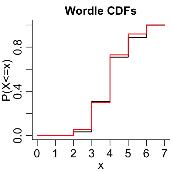
  • Let’s compare the CDFs of my score and my partner’s score.
y=Number of tries P(Y=y|\text{Simon}) P(Y=y|\text{Lillie})
1 0 0
2 0.03 0.05
3 0.28 0.24
4 0.40 0.44
5 0.18 0.19
6 0.11 0.08
Code
wordle1 = c(0, 2, 17, 25, 11, 7)
wordle2 = c(0, 2, 9, 16, 7, 3)
wordle1 = cumsum(wordle1/sum(wordle1))
wordle2 = cumsum(wordle2/sum(wordle2))
x = 0:7
plot(x, c(0,wordle1, 1), main='Wordle CDFs', type='s', ylab='P(X<=x)')
points(x, c(0,wordle2, 1), type='s', col='red')

Code
main = c()
  • What is the interpretation of this graph?
  • Who is doing better (getting the word in fewer guesses)?

Mean

  • The mean might be a nicer way to compare our scores.

The mean is the most common expected value

\mathbb{E} X = \int_{-\infty}^\infty x p(x) dx = \sum_{x}x p(x).

  • The integral notation is in the sense of “real analysis” type integrals that can refer to sums or integrals. This is to emphasize that the definition is the same with continuous or discrete random variables.
y=Number of tries P(Y=y|\text{Simon}) P(Y=y|\text{Lillie}) y\times P(Y=y|\text{Lillie or Simon})
1 0 0
2 0.03 0.05
3 0.28 0.24
4 0.40 0.44
5 0.18 0.19
6 0.11 0.08
  • \mathbb{E}X is a nonrandom value, called a parameter.
  • A parameter is something that describes a feature of the distribution of a random variable.
  • For the Bernoulli distribution, p.
  • For multinomial, it’s the vector of probabilities.
  • For the normal distribution

\mathbb{E} X = \int_{-\infty}^\infty x \frac{1}{\sqrt{2\pi} \sigma} e^{-\frac{1}{2\sigma^2} (x - \mu)^2} dx = \mu.

  • Properties include
    • \mathbb{E}\{ aX + b Y\} = \{ a\mathbb{E}X + b \mathbb{E}Y\}, for constant values a and b.

Variance

  • Another common expectation is the variance

\text{Var}(X) = \mathbb{E} (X - \mathbb{E}X)^2 = \mathbb{E} X^2 - (\mathbb{E} X)^2

  • In words, it is the average squared distance of the random variable from its expected value.

  • It is a measure of the amount of spread of a random variable

  • For the normal distribution

\mathrm{Var}( X ) = \int_{-\infty}^\infty (x-\mu)^2 \frac{1}{2\pi \sigma^2} e^{-\frac{1}{2\sigma^2} (x - \mu)^2} dx = \sigma^2.

  • Properties
    • \mathrm{Var}(bX-a) = b^2 \mathrm{Var}(X).

Wordle example

y=Number of tries P(Y=y|\text{Simon}) P(Y=y|\text{Lillie}) y\times P(Y=y|\text{Lillie or Simon})
1 0 0
2 0.03 0.05
3 0.28 0.24
4 0.40 0.44
5 0.18 0.19
6 0.11 0.08

Z-normalization

  • Given what we know about properties of mean and variance, we can standardize random variables
  • Assume \mathbb{E} X =\mu and \mathrm{Var}(X) = \sigma^2. What is the mean and variance of? (X-\mu)/\sigma
  • This is often applied to data using estimates z_i = (x_i - \bar x)/s
  • It makes your data mean zero and variance/SD equal to 1.

Aside: Mean and variance for random variables and datasets

  • The mean and variance formulas are very similar between datasets and random variables.

    • Mean (for discrete random variable):

    \mathbb{E} X = \sum_{x} x p(x)\\ \bar x = \frac{1}{n}\sum_{i=1}^n x_i

    • Variance (also for a discrete random variable)

    \mathrm{Var}(X) = \mathbb{E}\{(X - \mathbb{E}X)^2\} = \sum_x (x - \mathbb{E}X)^2 p(x) \\ s^2 = \frac{1}{(n-1)}\sum_{i=1}^n (x_i - \bar x)^2

  • This is just something to keep in mind when we are thinking about connecting the math we’re using to real data