Class 4

Objectives:

1. Learn about jointly distributed random variables
2. Learn to use probability to think about data
3. Learn to construct a confidence interval and test statistic

Review of mean and expectation

• Let’s find the mean and variance of a Bernoulli random variable.

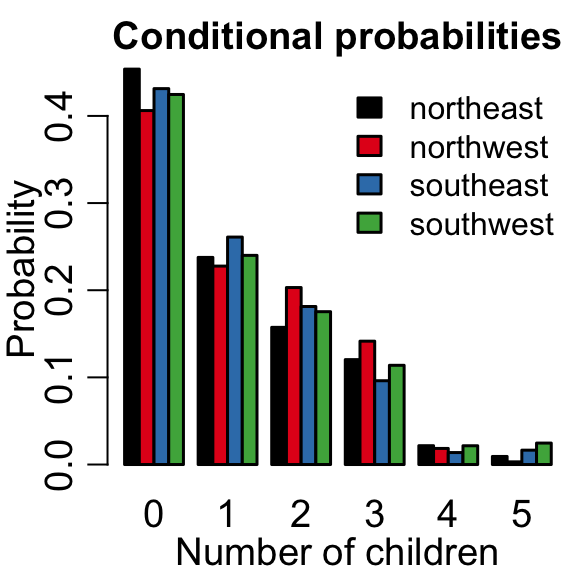
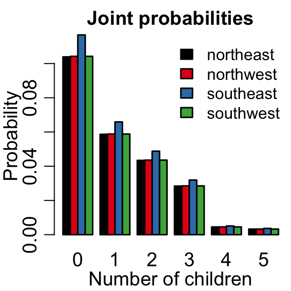
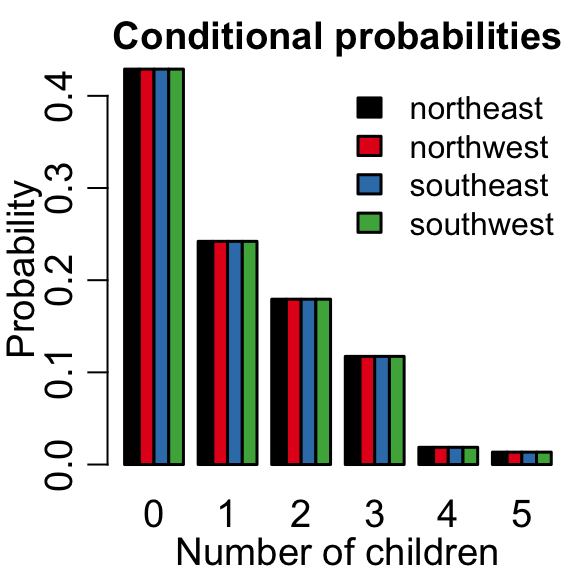
Jointly distributed random variables

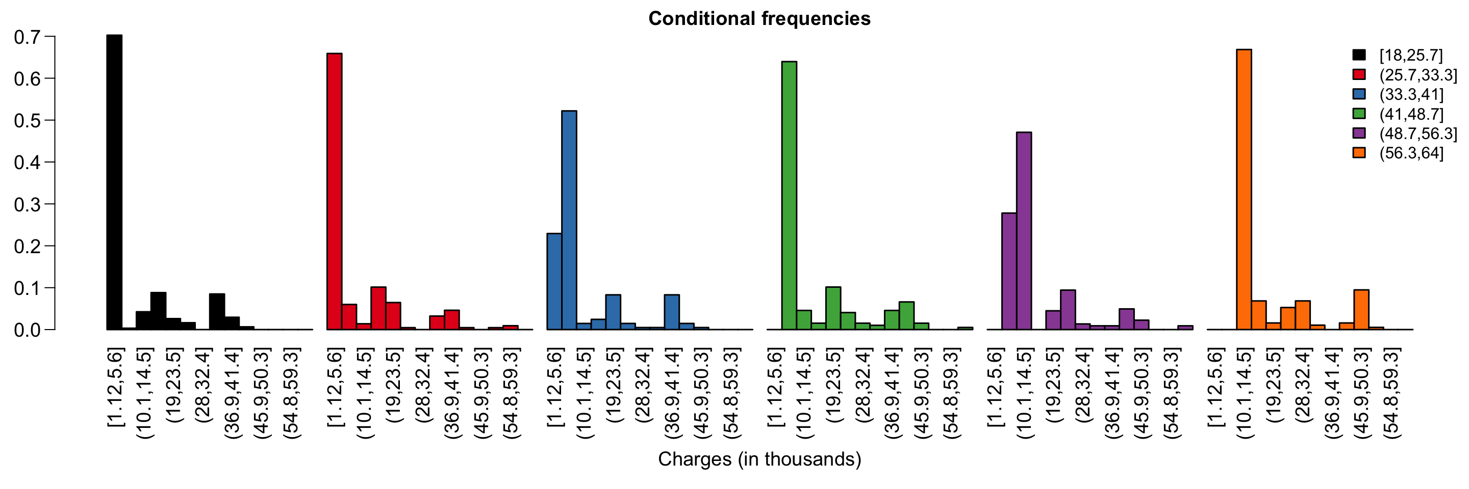
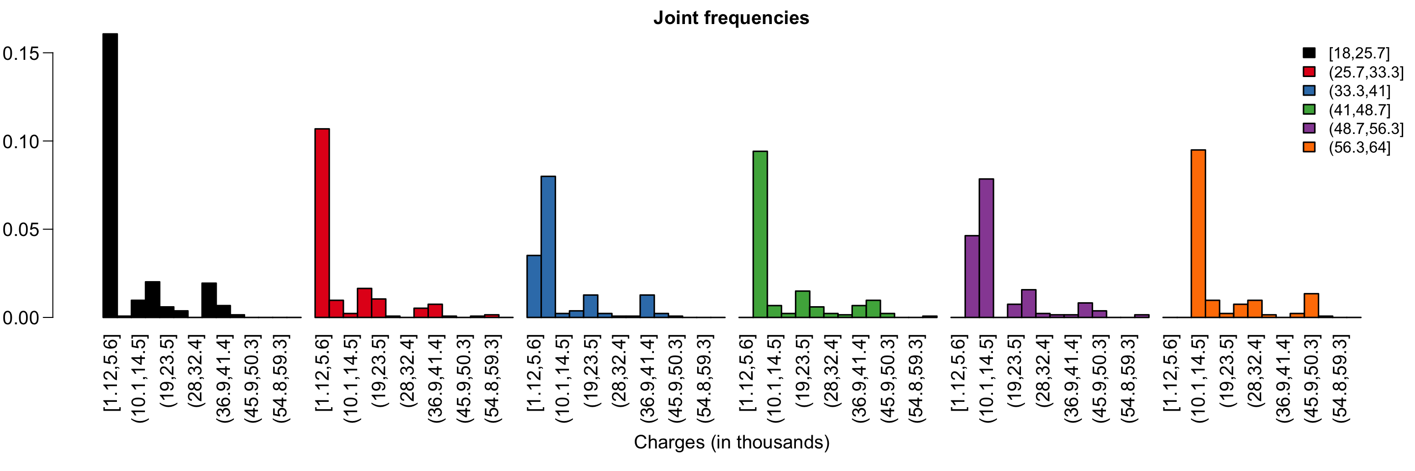
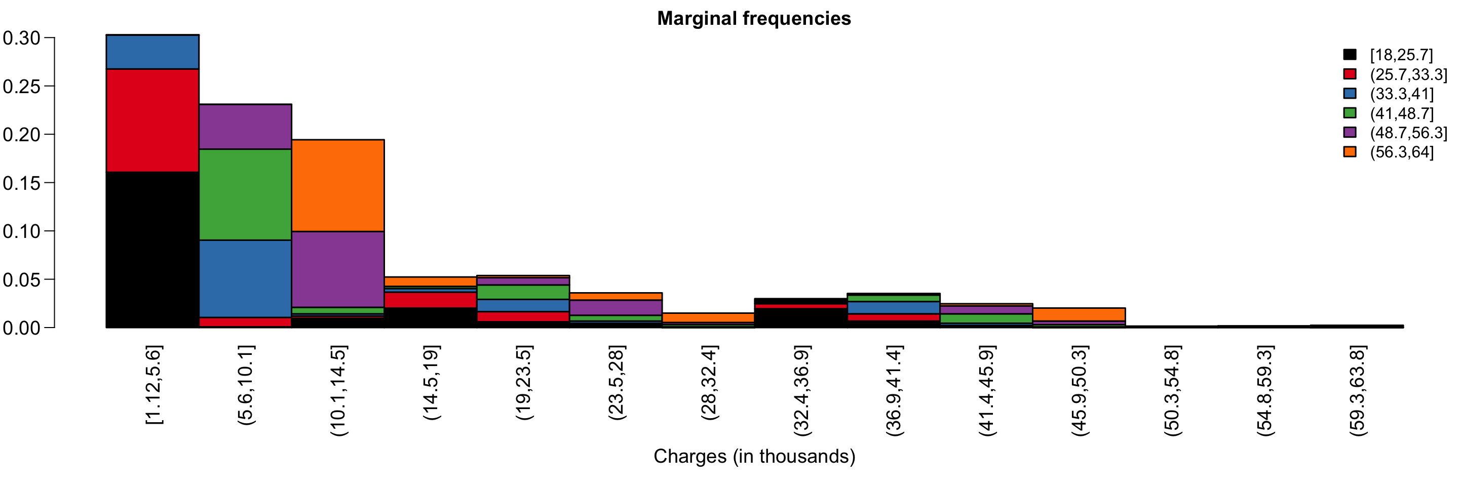
Jointly distributed random variables describe the probability of two things occurring. In the insurance dataset, we can consider the probability of having a certain number of children living in a certain area.

Code

library(RESI) # contains insurance dataset

Registered S3 method overwritten by 'clubSandwich':
  method    from    
  bread.mlm sandwich

Code

childByRegion = table(insurance$region, insurance$children)
childByRegion = childByRegion/sum(childByRegion)
knitr::kable(round(childByRegion, 2))

	0	1	2	3	4	5
northeast	0.11	0.06	0.04	0.03	0.01	0.00
northwest	0.10	0.06	0.05	0.03	0.00	0.00
southeast	0.12	0.07	0.05	0.03	0.00	0.00
southwest	0.10	0.06	0.04	0.03	0.01	0.01

• Let X be a random variable denoting number of children

  • Is it categorical/continuous/ordinal?

• Let Y be a random variable denoting region

  • Is it categorical/continuous/ordinal?

• joint distribution is a function of both variables \mathbb{P}(X=x, Y=y) = f(x,y).

• Questions about regional differences and number of children can be determined from the table

• What is the probability of having zero kids and living in the east?

• What is the probability of having zero kids?

Marginal probabilites

• Marginal probabilities are the probability of something occurring for one of the random variables, ignoring the other one.
• It’s called marginal, because you just add all the probabilities in the row or column and write it in the margin.

Conditional probabilities

• Conditional probabilities are to express statements dependent on something happening.
• Conditional probabilities are written \mathbb{P}(X=x \mid Y=y)
  • What is the probability of having three or more kids given living in the southeast? \mathbb{P}(X\ge 3 \mid Y=\text{``southeast"} )
  • What is the probability of living in the Northeast if you have one child?
• Conditional probability can be computed from the joint distribution \mathbb{P}(X=x\mid Y=y) = \mathbb{P}(X=x, Y=y)/\mathbb{P}(Y=y)

Code

condTab = sweep(childByRegion, 1, rowSums(childByRegion), FUN = '/')
knitr::kable(round(condTab, 2))

	0	1	2	3	4	5
northeast	0.45	0.24	0.16	0.12	0.02	0.01
northwest	0.41	0.23	0.20	0.14	0.02	0.00
southeast	0.43	0.26	0.18	0.10	0.01	0.02
southwest	0.42	0.24	0.18	0.11	0.02	0.02

Code

barplot(condTab, main='Conditional probabilities', ylab='Probability', xlab='Number of children', beside=T, col=cols[1:nrow(condTab)])
legend('topright', fill=cols[1:nrow(condTab)], legend=rownames(condTab), bty='n' )

Conditional expectations

• One you have conditional probabilities, you can do all the same stuff with it that you would do with a regular random variable
• For example, \mathbb{E}(X \mid Y) = \sum_{x} x f_{X\mid Y}(x \mid y)

Independence

• Two random variables are independent if they factor \mathbb{P}(X=x, Y=y) = \mathbb{P}(X=x)\mathbb{P}(Y=y) for all possible values of x and y.
• Intuitively, this means that fixing one variable doesn’t affect the distribution of the other.
• Another way to express it is that \mathbb{P}(X=x\mid Y=y) = \mathbb{P}(X=x).
• The table is pretty close to independent.

If the table above were perfectly independent, it might look like this:

Code

rs = rowSums(childByRegion)
cs = colSums(childByRegion)
indepTab = outer(rs, cs)
knitr::kable(round(indepTab, 3))

	0	1	2	3	4	5
northeast	0.104	0.059	0.043	0.028	0.005	0.003
northwest	0.104	0.059	0.044	0.029	0.005	0.003
southeast	0.117	0.066	0.049	0.032	0.005	0.004
southwest	0.104	0.059	0.044	0.029	0.005	0.003

Code

barplot(indepTab, main='Joint probabilities', ylab='Probability', xlab='Number of children', beside=T, col=cols[1:nrow(indepTab)])
legend('topright', fill=cols[1:nrow(indepTab)], legend=rownames(indepTab), bty='n' )

Code

condTab = sweep(indepTab, 1, rowSums(childByRegion), FUN = '/')
barplot(condTab, main='Conditional probabilities', ylab='Probability', xlab='Number of children', beside=T, col=cols[1:nrow(condTab)])
legend('topright', fill=cols[1:nrow(condTab)], legend=rownames(condTab), bty='n' )

Joint random variables in the insurance dataset

• Remember the relationship between age and charges in the insurance data

Code

library(RESI)
plot(insurance[,'age'], insurance$charges, ylab='Charges', xlab='Age', main=paste('Age', 'and', 'Charges') )

• The scatter plot can be thought of as a dataset version of a joint density f_{X,Y}(x,y)
• We can get the conditional histograms for a few different age groups

Code

par(mar=c(8,2.8,1.8,.2), mgp=c(6,.7,0))
nbin = 15
insCat = with(insurance, data.frame(age=cut(age, breaks = seq(min(age), max(age), length.out=7), include.lowest=T), charges=cut(charges/1000, breaks = seq(min(charges/1000), max(charges/1000), length.out=nbin), include.lowest=T) ) )
condTab = do.call(cbind, by(insCat$charges, insCat$age, function(x){res=table(x); res/sum(res)}))
barplot(condTab, beside=TRUE, col=rep(cols[1:ncol(condTab)], each=nbin-1),
        names.arg = rep(rownames(condTab), ncol(condTab) ), las=2, xlab='Charges (in thousands)', main='Conditional frequencies')
legend('topright', fill=cols[1:ncol(condTab)], legend=colnames(condTab), bty='n')

Code

par(mar=c(8,2.8,1.8,.2), mgp=c(6,.7,0))
nbin = 15
jointTab = do.call(cbind, by(insCat$charges, insCat$age, function(x){res=table(x); res}))
jointTab = jointTab/sum(jointTab)
barplot(jointTab, beside=TRUE, col=rep(cols[1:ncol(jointTab)], each=nbin-1),
        names.arg = rep(rownames(jointTab), ncol(jointTab) ), las=2, xlab='Charges (in thousands)', main='Joint frequencies')
legend('topright', fill=cols[1:ncol(jointTab)], legend=colnames(jointTab), bty='n')

Code

par(mar=c(8,2.8,1.8,.2), mgp=c(6,.7,0))
nbin = 15
test = barplot(t(jointTab), beside=FALSE, col=cols[rep(1:ncol(jointTab), nbin-1)], las=2, xlab='Charges (in thousands)', main='Marginal frequencies', space=0)
legend('topright', fill=cols[1:ncol(jointTab)], legend=colnames(jointTab), bty='n')

Connecting data and probability with a random sample

Statistics is a way to learn about the world from a data set

For now, let’s work with the question, “What is the proportion of people in the United States who smoke cigarettes?”

• We’ll define currently smoking cigarettes as anyone who has smoked at least one in the last 30 days.
• One way to answer this question is to ask everyone in the US whether the smoke.
• Another way is to ask a random sample of people whether they smoke.
  • How do we know that the proportion from the random sample is close to the proportion in the population?
  • Probability is the tool we use to tie information from our sample to the population we want to learn about.
• In this example, we can assume people from the US are sampled randomly and that each person’s answer is X_i \sim \text{Be}(p)
• If we repeated this for n independently sample people, X_1, \ldots, X_n is called a random sample.

There are three objects here:

1. p - the unknown parameter
2. X_1, \ldots, X_n - the random sample, which can be use to compute an estimator.
3. x_1, \ldots, x_n - the observed data, which can be used to compute and estimate.

Let’s see what this looks like in a simulation. A simulation lets us create a very simple fake world, where we know parameters, which we are usually not able to know.

Code

nsduh = readRDS('nsduh/puf.rds')

# Pretend that the NSDUH dataset is the entire population of
# the united states -- There are n=56,897 people in the US.
table(nsduh$cigmon)

   no   yes 
46209 10688 

Code

# This is the parameter that we usually don't get to see.
# We can only see it here, because we are pretending that
# the NSDUH data is the full population of the US.
p = mean(nsduh$cigmon=='yes')
p

[1] 0.1878482

Code

# The sample size we choose.
n = 50
# Capital X represents a random sample from the population.
# This is just a statistical concept that tells us what would
# happen if we repeated the experiment a whole bunch of times.
#
# run X() at the command line multiple times to see that it
# it changes each time
X = function(n=50) sample(nsduh$cigmon, n, replace = TRUE)
X(n)

 [1] no  no  yes no  no  no  no  no  no  no  yes no  no  no  no  no  no  yes no 
[20] yes no  yes yes no  no  no  no  yes no  yes no  no  no  no  no  no  no  no 
[39] no  no  no  no  no  no  no  no  no  no  yes no 
Levels: no yes

Code

X(n)

 [1] no  no  yes no  no  no  yes no  no  no  no  no  no  no  no  no  no  no  no 
[20] no  no  no  no  yes no  no  no  no  no  yes no  no  no  no  no  no  no  no 
[39] no  yes no  no  no  no  yes no  yes no  no  no 
Levels: no yes

Code

X(n)

 [1] no  no  no  no  no  no  no  no  yes no  no  no  no  no  no  no  no  yes no 
[20] no  no  yes no  no  yes no  no  no  no  no  no  yes no  no  no  no  no  no 
[39] no  no  no  no  yes no  no  no  no  yes no  no 
Levels: no yes

Code

# x is our observed data, it is not random, but we assume it was
# drawn as a random sample from the population
x = X(n)
x

 [1] no  no  yes no  yes yes no  no  no  yes no  no  no  no  yes no  no  yes no 
[20] no  no  no  no  no  yes no  no  no  no  no  no  no  no  no  no  yes no  yes
[39] no  no  no  no  no  no  no  no  no  yes no  no 
Levels: no yes

Code

# it does not change each time
x

 [1] no  no  yes no  yes yes no  no  no  yes no  no  no  no  yes no  no  yes no 
[20] no  no  no  no  no  yes no  no  no  no  no  no  no  no  no  no  yes no  yes
[39] no  no  no  no  no  no  no  no  no  yes no  no 
Levels: no yes

Code

x

 [1] no  no  yes no  yes yes no  no  no  yes no  no  no  no  yes no  no  yes no 
[20] no  no  no  no  no  yes no  no  no  no  no  no  no  no  no  no  yes no  yes
[39] no  no  no  no  no  no  no  no  no  yes no  no 
Levels: no yes

• Statistics tries to learn about the parameter p, using only the data x, by studying the mathematical properties of X.
• X can tell us features about what would happen if we ran an experiment a whole bunch of times.

Mathematically

Parameters

• Usually a parameter is defined based on the interest of the clinician and from the model for your data.
  • In this case, we assumed that each participant has a random probability of smoking with probability p.

Estimates

Note, an estimate is a function of the observed sample and it is nonrandom (Why is it non random?). We often use lowercase letters to make that clear \bar x = n^{-1} \sum_{i=1}^n x_i.

Estimators

An estimator is a function of a random sample. The goal (usually) is to estimate a parameter of interest (here, p). Let’s consider the estimator \hat p = \bar X = n^{-1} \sum_{i=1}^n X_i, which we determine is pretty reasonable since \mathbb{E} \bar X = p.

• We can study the properties of estimators to learn about how they behave.
• If we like an estimator we can compute an estimate using our sample.
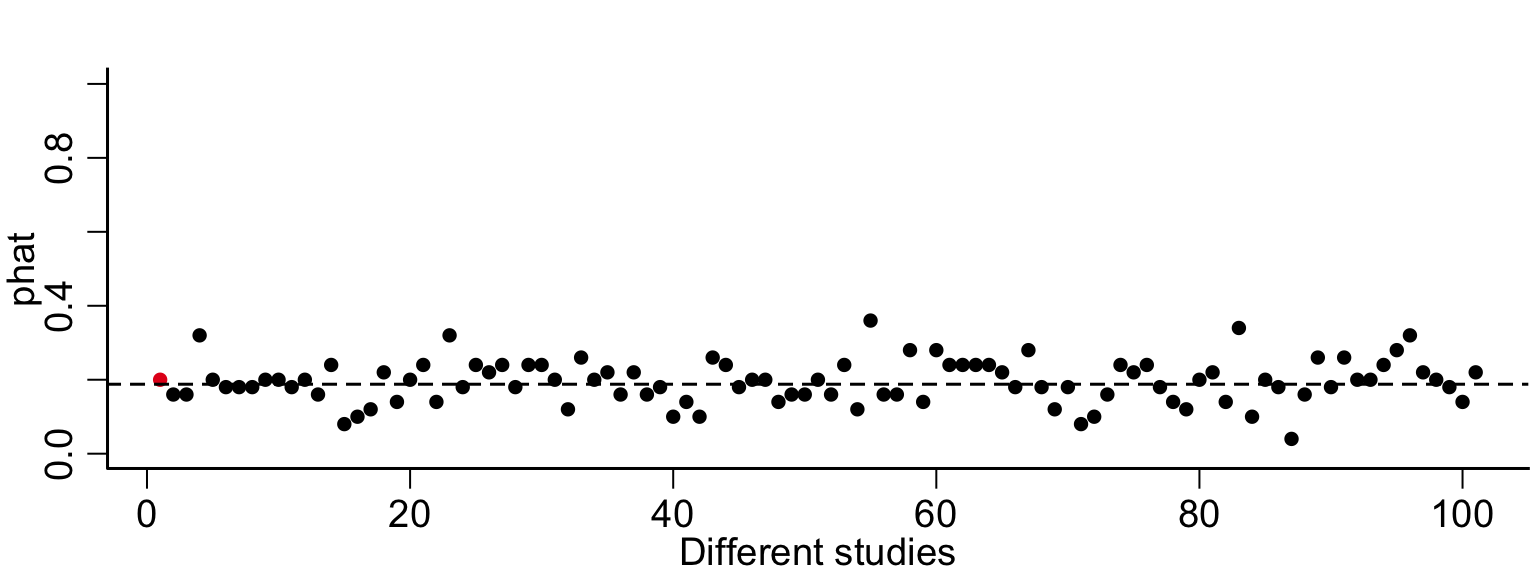
• We can use features of our estimator to make probabilistic statements about what might happen if we repeat our study. Dataset-to-dataset variability

We can start to think about properties of the estimator to understand what it looks like if I were to repeat a study a whole bunch of times

• What is the mean of the estimator?
• What is the variance of the estimator?

Why do we care about this? Because we want to know the probability that our estimator is close to the value in the population.

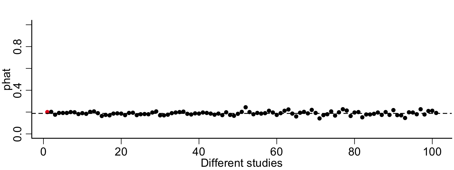
Code

n=50
# p is the unknown parameter.
p = mean(nsduh$cigmon=='yes')
# this is the data we collected, it was a random sample from the population
x = X(n)
# this is the proportion of smokers we observed
phatObs = mean(x=='yes')
# this is an estimate the variance of the estimator phat
Var_phat = phatObs * (1-phatObs)/n



# How can we tell where p is if we don't get to see it?


# We can't know for sure, but we can see how often the random variable version of phat is close to p
nstudies = 100
phats = rep(NA, nstudies)
for(i in 1:nstudies){
  phats[i] = mean(X(n)=='yes')
}
plot(c(phatObs, phats), xlab='Different studies', ylab='phat', ylim=c(0,1), col=c(cols[2], rep(cols[1], nstudies)) )
abline(h=p, lty=2)

Code

# because phatObs was created the same way as the phat

Code

n=500
# p is the unknown parameter.
p = mean(nsduh$cigmon=='yes')
# this is the data we collected, it was a random sample from the population
x = X(n)
# this is the proportion of smokers we observed
phatObs = mean(x=='yes')
# this is an estimate the variance of the estimator phat
Var_phat = phatObs * (1-phatObs)/n



# How can we tell where p is if we don't get to see it?


# We can't know for sure, but we can see how often the random variable version of phat is close to p
nstudies = 100
phats = rep(NA, nstudies)
for(i in 1:nstudies){
  phats[i] = mean(X(n)=='yes')
}
plot(c(phatObs, phats), xlab='Different studies', ylab='phat', ylim=c(0,1), col=c(cols[2], rep(cols[1], nstudies)) )
abline(h=p, lty=2)

Code

# because phatObs was created the same way as the phat

Some common statistical jargon so far

Types of variables

• Categorical variable - a variable that takes discrete values, such as diagnosis, sex,
• Continuous variable - a variable that can take any values within a range, such as age, blood pressure, brain volume.
• Ordinal variable - a categorical variable that can be ordered, such as age category, Likert scales, Number of days, Number of occurrences.
• Discrete random variable - takes integer values.
• Continuous random variable - takes real values.

Distribution/Density features

• Mode/ Non-modal/Unimodal/ Bimodal - a peak in a density.

  • Non-modal - no peak
  • Unimodal - one peak
  • Bimodal - two peaks

• Quantile - the pth quantile, q_p divides the distribution such that p% of the data are below q_p.

  • Median - 50th quantile of a distribution

• Skew/Skewness - the amount of asymmetry of a distribution

  • Symmetric distribution - a distribution with no skew

• Kurtosis - the heavy tailed-ness of a distribution.

• Probability Density/Mass Function - function, f_X, that represents f_X(x) = \mathbb{P}(X=x)

• Cumulative Distribution Function - function, F_X that represents F_X(x) = \mathbb{P}(X\le x)

• Parameter – Target unknown feature of a population (nonrandom)

• Estimate – Value computed from observed data to approximate the parameter (nonrandom)

• Estimator – A function of a random sample to approximate the parameter