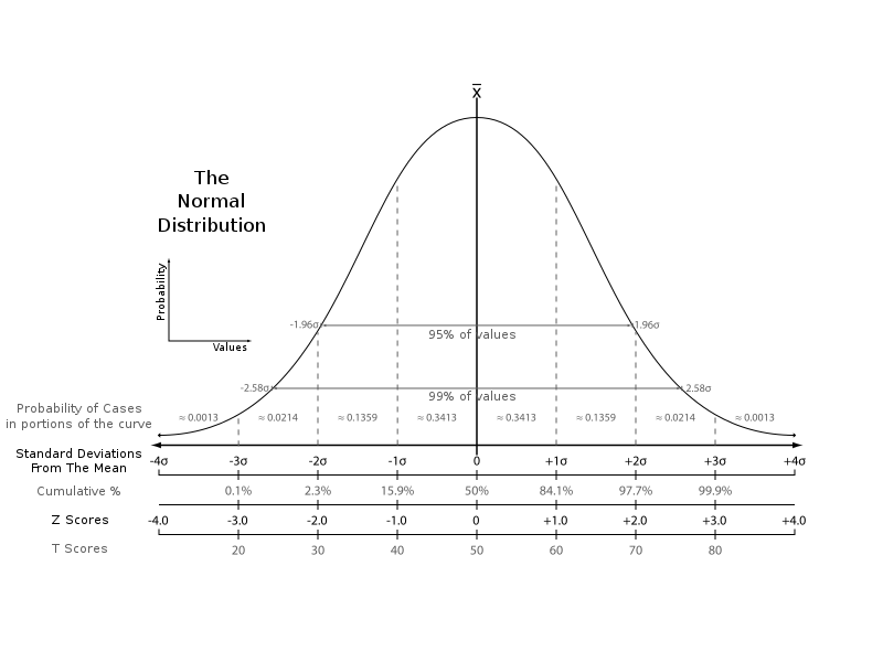
Standard normal Z\sim N(0,1) often denoted with a Z.
PDF often denoted by \phi(z).
CDF often denoted by \Phi(z).
For Y \sim N(\mu, \sigma^2), (Y-\mu)/\sigma \sim N(0, 1) (often called Z-normalization).
\mathbb{P}(\lvert Z \rvert\le 1.96) = \Phi(1.96) - \Phi(-1.96) \approx 0.95.
\mathbb{P}( Z \le 1.64) = \Phi(1.64) \approx 0.95.
The Central Limit Theorem
The Central Limit Theorem (Durrett, pg. 124): Let X_1, X_2, \ldots be iid with \mathbb{E} X_i = \mu and \text{Var}(X_i) = \sigma^2 \in (0, \infty).
If \bar X_n = n^{-1} \sum_{i=1}^n X_i, then
n^{1/2}(\bar X_n - \mu)/\sigma \to_D X,
where X \sim N(0,1).
Comments:
We need the variance to be finite (stronger assumptions than LLN)
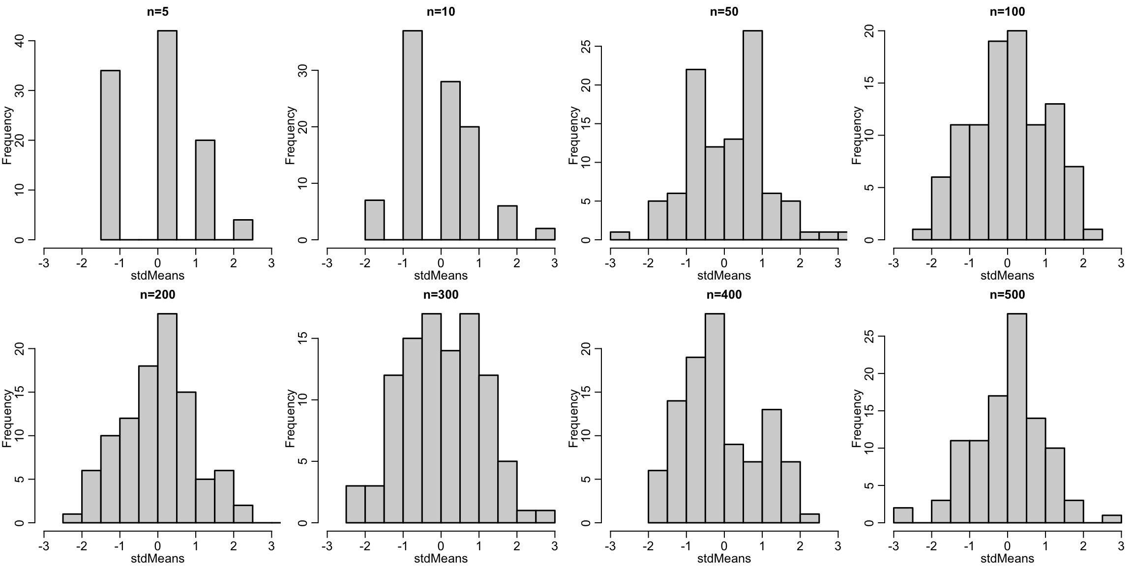
In words the central limit theorem means that no matter what the distribution of the data are, the mean will always me normally distributed in large samples.
More specifically, (\bar X - \mu)/\sigma will be standard normal
Conceptual overview
This is to illustrate the CLT numbers using some example data to answer the question, “What is the proportion of people in the United States who smoke cigarettes?”
We’re again pretending that the NSDUH dataset is the entire population of the US.
Code
# read in datansduh =readRDS('nsduh/puf.rds')# ever tried cigarettes indicatortriedCigs = nsduh$cigmon# make it a Bernoulli random variabletriedCigs =ifelse(triedCigs=='yes', 1, 0)mu =mean(triedCigs)sigma =sqrt(var(triedCigs))ns =c(5, 10, 50, 100, 200, 300, 400, 500)# for each sample size, we performing 100 studiesstudies =1:100layout(matrix(1:8, nrow=2, byrow=TRUE))for(n in ns){# Each person in the class is performing a study of smoking studies =lapply(studies, function(studies) sample(triedCigs, size=n))names(studies) = studies# get the mean for each person's study studyMeans =sapply(studies, mean) stdMeans =sqrt(n)*(studyMeans - mu)/sigma# histogram of the study meanshist(stdMeans, xlim =c(-3,3), breaks=10, main=paste0('n=', n))}
Constructing confidence intervals
We can use the normal distribution to compute confidence intervals
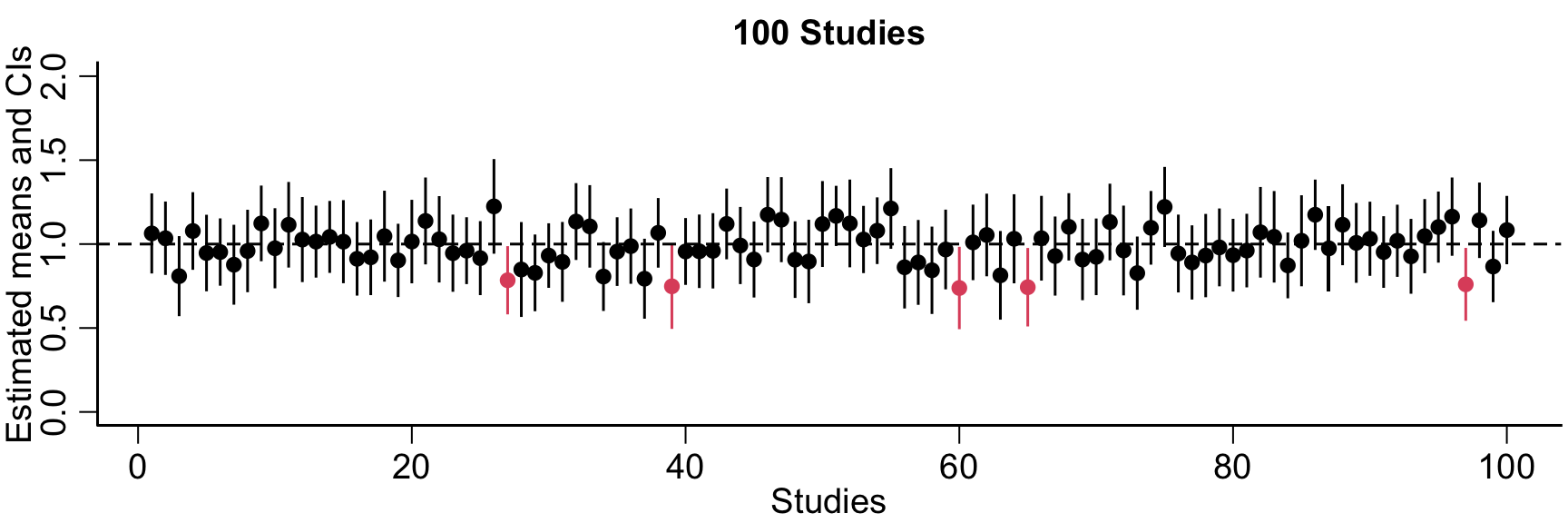
Confidence intervals are an interval obtained from a random sample that contains the true value of the parameter with a given probability.
P\{L(X_1, \ldots, X_n) \le p < U(X_1, \ldots, X_n) \} = 1-\alpha,
for a given value \alpha \in (0,1).
Note what things are random here (the end points). The parameter is fixed.
It comes from the fact that (\bar X - \mu)/\sigma \sim N(0,1) (approximately).
The interpretation is that the procedure that creates the CI captures the true parameter 1-\alpha% of the time.
Dataset-to-dataset variability
Code
mu =1sigma =0.8n =50nsim =100alpha =0.05CIs =data.frame(mean=rep(NA, nsim), lower=rep(NA, nsim), upper=rep(NA, nsim))for(sim in1:nsim){# draw a random sample X =rnorm(n, mean=mu, sd=sigma) stdev =sd(X)# construct the confidence interval CIs[sim, ] =c(mean(X), mean(X) +c(-1,1)*qnorm(1-alpha/2)*stdev/sqrt(n))}CIs$gotcha =ifelse(CIs$lower<=mu & CIs$upper>=mu, 1, 2)# range(c(CIs$lower, CIs$upper))plot(1:nsim, CIs$mean, pch=19, ylim =c(0,2), main=paste(nsim, 'Studies'), col=CIs$gotcha, ylab='Estimated means and CIs', xlab='Studies' )segments(x0=1:nsim, y0=CIs$lower, y1=CIs$upper, col=CIs$gotcha)abline(h=mu, lty=2 )
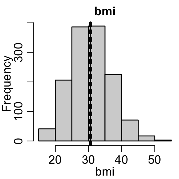
Computing a confidence interval in real data
We can compute confidence intervals more generally (not just for proportions or means)
Examples
Code
library(RESI)
Registered S3 method overwritten by 'clubSandwich':
  method    from
  bread.mlm sandwich
Code
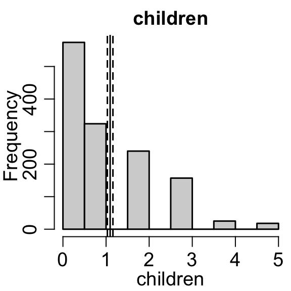
var ='bmi'mu =mean(insurance[,var])CI = mu +qnorm(c(0.025, 0.975)) *sd(insurance[,var])/sqrt(length(insurance[,var]))hist(insurance[,var], main=var, xlab=var)abline(v=mu)abline(v=CI, lty=2)
    Welch Two Sample t-test

data:  charges by smoker
t = -32.752, df = 311.85, p-value < 2.2e-16
alternative hypothesis: true difference in means between group 0 and group 1 is not equal to 0
95 percent confidence interval:
 -25034.71 -22197.21
sample estimates:
mean in group 0 mean in group 1
       8434.268       32050.232
Some common statistical jargon so far
Types of variables
Categorical variable - a variable that takes discrete values, such as diagnosis, sex,
Continuous variable - a variable that can take any values within a range, such as age, blood pressure, brain volume.
Ordinal variable - a categorical variable that can be ordered, such as age category, Likert scales, Number of days, Number of occurrences.
Discrete random variable - takes integer values.
Continuous random variable - takes real values.
Distribution/Density features
Mode/ Non-modal/Unimodal/ Bimodal - a peak in a density.
Non-modal - no peak
Unimodal - one peak
Bimodal - two peaks
Quantile - the pth quantile, q_p divides the distribution such that p% of the data are below q_p.
Median - 50th quantile of a distribution
Skew/Skewness - the amount of asymmetry of a distribution
Symmetric distribution - a distribution with no skew
Kurtosis - the heavy tailed-ness of a distribution.
Probability Density/Mass Function - function, f_X, that represents f_X(x) = \mathbb{P}(X=x)
Cumulative Distribution Function - function, F_X that represents F_X(x) = \mathbb{P}(X\le x)
Parameter – Target unknown feature of a population (nonrandom)
Estimate – Value computed from observed data to approximate the parameter (nonrandom)
Estimator – A function of a random sample to approximate the parameter