Modern Topics
Centile estimation
Brain charts for the human lifespan
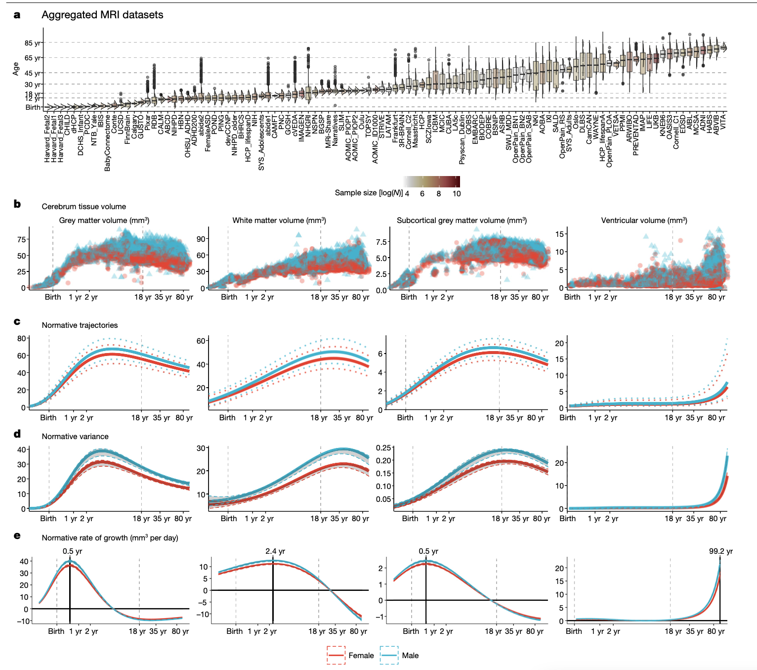
- Bethlehem & Siedlitz et al. used a massive data set(over 100,000 participants) to fit “normative” trajectories across the lifespan.
- They used generalized additive models for location, scale, and shape (GAMLSS).
- They used random effects terms to account for scanner differences across sites.
Centiles
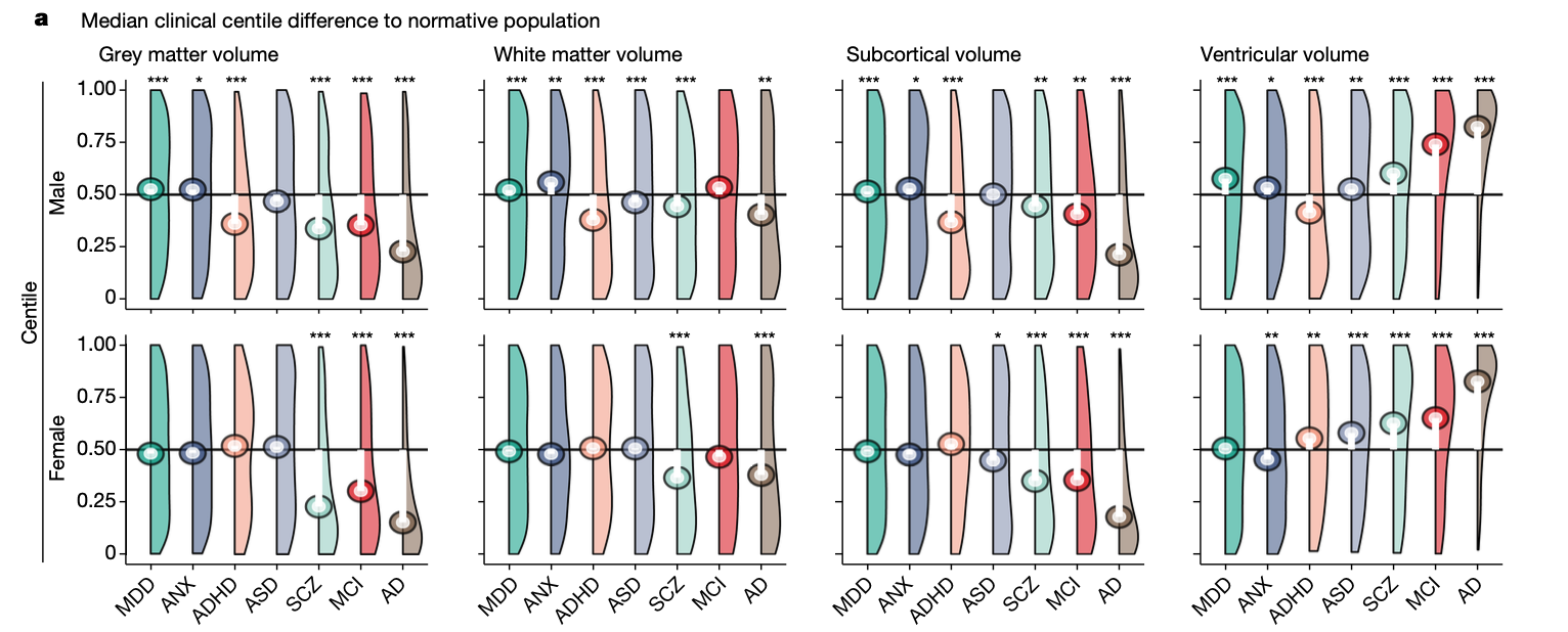
They then used the normative curves to estimate where people fall relative to someone of the same age and sex. For a new observation \(y_j\), their centile is \[ \mathbb{P}(Y \le y_j\mid \text{age}_j, \text{sex}_j, \text{site}_j, \text{software}_j) \]
Instead of conducting analyses relative to a control group, they compared the median of the centile values to 0.5.
- It’s possible this improves power, because the full sample used to construct the GAMLSS models acts (heuristically) as the control group
Multivariate centiles
- This whole GAMLSS/centile approach was repeated for every region in the Desikan-Killiany brain atlas.
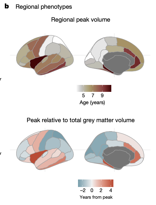
- Then they computed multivariate centiles across all these regions.
- Multivariate centiles were computed as follows.
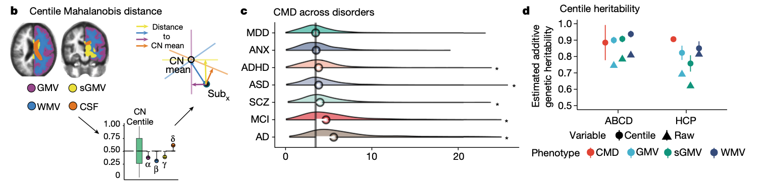
1. Multivariate centiles
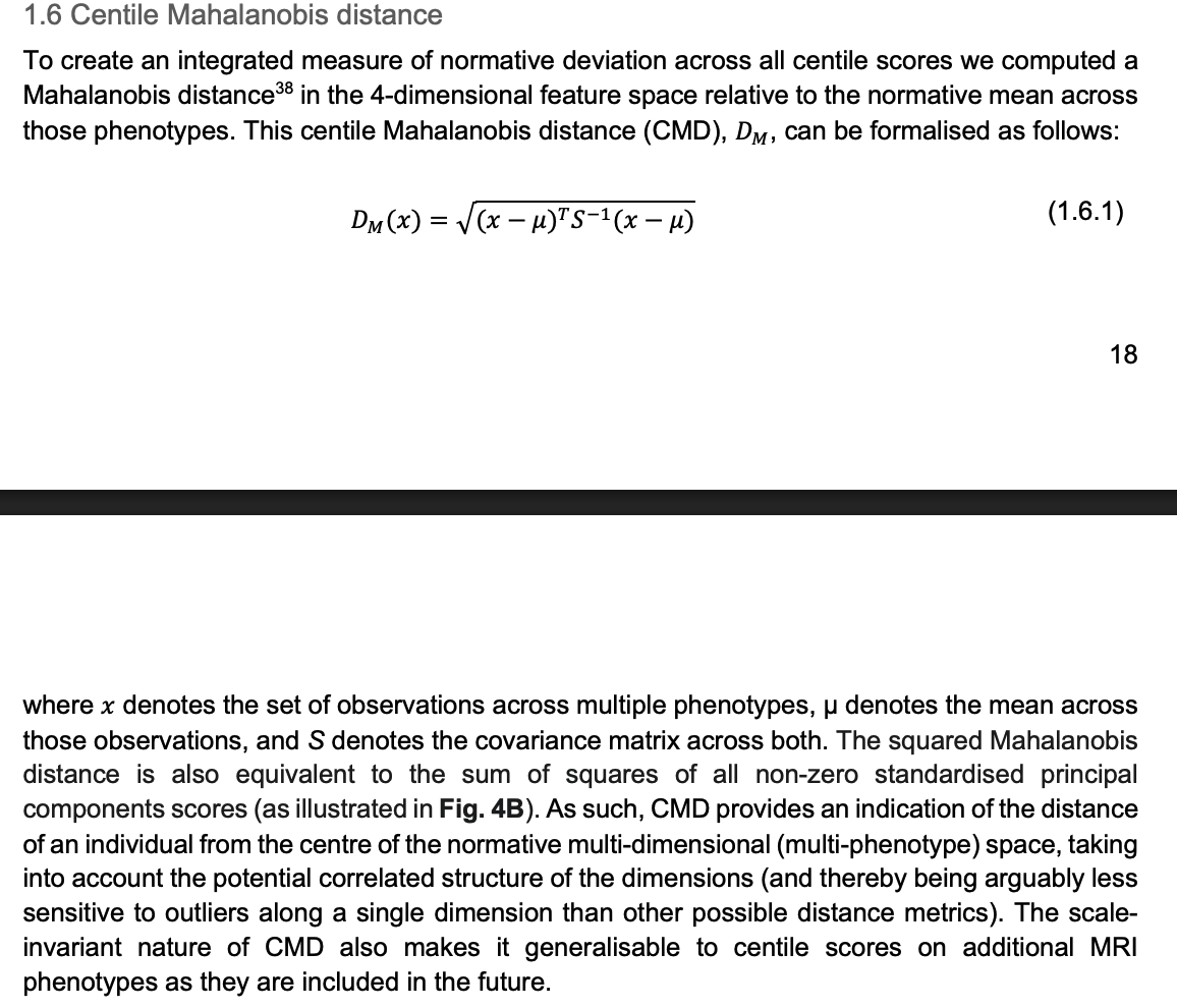
- Since the beginning, there’s been interest multivariate centiles, that provide a single value to summarize a person’s overall deviance from the population.
- The initial proposed methods to do this are unusual because they compute a Mahalanobis distance on the centile scale.
- Goal: Develop and evaluate a method that transforms the centiles to a multivariate normal, computes centiles based on the distance to the center of the distribution and back-transforms to the centile scale.
2. Centile estimation in multilevel models
- Multi-level models are needed for centile estimation:
- To adjust for technical (site/hardware/software) effects.
- To use multiple measurements from the same individual.
- We use random effects models (GAMLSS) to account for the correlation among measurements.
- Different approaches are needed to account for these repeated measurements:
- For site effects, we want to estimate and remove these effects when computing centiles in a new dataset.
- For person/family random effects, people aren’t really sure how to handle them. I think we want to compute centiles marginally.
- Goal: Figure out how to correctly estimate centiles from models with person/family random effects.
- First, you will have to define what “correctly” means, i.e. what is the centile value we would want to estimate.
- Then you have to figure out how to compute it for a new observation from a fitted model.
Confidence set estimation
3. Confidence sets for a fixed effect size
- Xinyu’s confidence sets invert simultaneous confidence intervals and work for all effect size thresholds.
- If people are only interested on one particular threshold, then these can be conservative.
- Methods exist for a single effect size threshold.
- Goal: Apply these methods to the robust effect size index and write code to implement it.
Bowring paper overview
- Bowring et. al. 2021 implemented the single-threshold confidence set method for Cohen’s \(d\) effect size.
- Their bootstrap procedure was more complicated than ours needs to be (we have a valid bootstrap already).
- You will need to understand and implement the method they use.
4. FDR controlling confidence sets
- Xinyu’s method creates confidence sets that control the FWER.
- Many people like to control the FDR instead, because it is less conservative.
- Goal: Implement a confidence set method to control the FDR for the RESI for a single threshold.
- Do a literature search for this, because I know people are thinking about it already.
- I think for a given threshold \(s\), it is similar to performing a test \(H_0(v): S(v) = s\).
- I’ve talked to a colleague, and they suggested you need to do it separately for the upper and lower sets \[ \begin{align*} H_0(v) & : S(v) \ge s \\ H_0(v) & : S(v) \le s \\ \end{align*} \]
Machine learning in neuroimaging
5. Apply CNNs for brain-phenotype associations
- Megan evaluated common ML models in her paper.
- Convolution neural networks are more flexible and can incorporate spatial information.
- Goal: Evaluate whether there is improved accuracy in predicting age and psychopathology variables in the RBC dataset.
- Goal: Evaluate validity of Megan’s semiparametric one-step estimator when using a CNN.
Background for CNNs
- Good for image input. Can be used for phenotype prediction with sample sizes we have in neuroimaging? I’m not sure.
- Review by Mienye et al. 2025
- I’m no expert, but see if this is feasible.
6. Improved accuracy of confidence intervals
- Confidence interval coverage in “small” samples is still below nominal level using Megan’s methods
- Low coverage is due to finite-sample bias and the contribution of high-order terms in the Taylor expansion
- Goal: investigate approaches to improve small sample coverage
- “Normalizing transformations”
- Incorporating higher-order terms in the Taylor expansion
- Using simulations
Replicability
Huge concern in neuroimaging
Definition of replicability
- Replicability is often defined in terms of the \(p\)-value. In this case, replicability is related to type 1 error and power.
- A more sensible approach, might be to define replicability in terms of the MSE of an effect size (vector across all \(V\) image locations)
\[ \mathbb{E} \lVert \hat S - S \rVert^2/V \]
- Tangential math: For two independent samples the expected distance of their effect size (vectors across all image locations)
\[ \mathbb{E} \lVert \hat S_1 - \hat S_2 \rVert^2 = 2 \mathrm{tr}\{\mathrm{Var}(\hat S_1)\} \] *
7. Evaluate an alternative approach for mass-univariate analysis
- Mass-univariate inference might have pretty low replicability
- We’ve been exploring ecological methods (RDA) to fit a mass-univariate model across the whole-brain together using dimension reduction.
- Imagine the mass-univariate analysis as a multivariate model \[ \mathbb{E} Y = X \beta \]
- where \(Y \in \mathbb{R}^{n \times V}\), \(X \in \mathbb{R}^{n \times m}\), \(\beta \in \mathbb{R}^{m \times V}\)
- RDA does dimension reduction within the modeling framework.
- It would be interesting to evaluate its MSE, bias, and variance relative to mass-univariate analysis to see whether it is better. My hypothesis is that is has better MSE due to lower variance and introducing some bias.
Project administration
Rank the projects
- Questions about the projects?
- Rank the projects using the google form
Project organization
- Organize your project like a statistical methods paper:
- Introduction
- Methods
- Results
- Analysis
- Discussion
- References
- Introduction should include
- Background contextualizing the problem and why it is important (including relevant literature).
- Example of how this problem arises in data analysis. The best example, is one from the dataset you will analyze in your paper.
- A literature review describing what’s been done to try to address the problem, and why it is inadequate.
- A description of your method and why it addresses the problem better than existing methods.
- Methods should include
- The dataset and what the goal of the analysis is.
- Comparator methods.
- Notation/Theory/Description of your method.
- Evaluation approach (usually includes some simulations). What are the metrics for evaluation?
- Results
- Simulation analysis results.
- Analysis results for your example.
- Discussion
- One paragraph recap.
- A paragraph for each important implication.
- Conclusion paragraph: take-home message of your paper.
Project grading
The idea is that you can fill in all aspects of the paper outline at a shallow depth. I’m expecting you work 4-8 hours a week including class time. When I grade your submission, I’ll think about these things:
- Continued effort
- Each Friday, submit less than a page progress that week separately for each team member. It can include code snippets, screenshots, figures, photos of math/theory, etc.
- No “dead-ends.” Your project as planned beginning of November may fail. You should re-direct/simplify if you hit a dead-end.
- Introduction
- Contextualized the problem
- Contextualized the importance
- Described the existing methods
- Summarized your approach and the gap it addresses
- Methods
- Your approach is logical statistically. i.e., it’s neat, not unnecessarily complicate and addresses the problem.
- Your approach and metrics for evaluation are valid.
- The methods you develop are actually valid for your example problem.
- Results
- Your results are presented neatly in figures that are easy to read.
- Discussion
- Your conclusions about the results is correct/justified.
- Clearly written
- ChatGPT writes TOO MUCH. Your writing should be as short and accessible as possible. The best writing makes your idea seem obvious and simple.
- Submission
- Submit your code and
.qmdfile and compiled html or pdf.
- Submit your code and
- Author contributions
- Every author should contribute. You will get a shared grade based on the final submission and presentation and a separate grade based on your weekly update.
Computing
- You will need access to computing and data.
- Depending on the project, it’s probably easiest if I give you access to my servers.
- We will figure that out after you choose projects.